11 Time Series Forecasting

Note

This is an EARLY DRAFT.

Time series forecasting is one setting in which economists are directly interested in making predictions. We have a series of observations of some set of variables over time, and we need to use them to predict the value of some variables in the future. Macroeconomic forecasting for the government, forecasting the income of a household to measure income shocks, or demand forecasting for a firm, all fall within the broad framework of time series forecasting.

Forecasting is a wide subject with a variety of sub-problems and approaches. It has been studied for a century, if not more. There is no way in which a single chapter can even broadly survey the whole area. Therefore in this chapter I have chosen to show a few things that capture the feel of current machine learning practice in this area. In the end we mention some of the important things we have left out and provide references.

11.1 Using standard tabular models for forecasting

Consider a simple forecasting problem in which we are given past values \(y_1, \dots, y_t\) of some variable and have to predict the next value \(y_{t+1}\). A prediction function for this problem will look like \[ \hat y_{t+1} = f_t(y_1,\ldots,y_t) \]

But this is just a standard regression problem, except that:

It is a different problem for each \(t\), as indicated by the \(t\)-subscript on \(f\). This is for two reasons. First, the input space keeps changing with \(t\). At \(t=2\) the input space is \((y_1,y_2)\) whereas at \(t=3\) it becomes \((y_1,y_2,y_3)\). As time passes, we have longer and longer history to work with. Second, in general the behaviour of the process generating \(y\) may depend on time (in the language of statisticians, it could be nonstationary). For example, if \(y_t\) is the number of leisure hours available to an individual at age \(t\), we might expect it to follow a U-shaped curve—high in childhood, low in working age, high again in retirement.
The regressors are not different variables, they are observations at different points of time of the same real-world ‘variable’. We might hope that there may be a commonality in how they contribute to predicting \(y_{t+1}\) which would be lost if we apply a general regression method to this problem.
We may have knowledge from outside the data of how the system generating the data may behave over time. One vary important example is that of seasonality. If \(y_t\) is the sale of ice-cream on date \(t\), we would expect it to follow a rough annual cycle, peaking in summer and falling-off in winter. It should be possible to incorporate this knowledge in our model.

These considerations may make you think that forecasting would be better served by models specialised for time-series tasks instead of general regression models. This was indeed the case till recently. However this intuition seems to have been overturned of late due to the increasing sophistication of general machine learning models, the increasing availability of data and increasingly complex processes that we wish to forecast. The best performing forecasting models right now are either general tabular regression models like LightGBM or MLPs or general tabular regression models which have only been tweaked slightly for the specifics of time-series forecasting.

To use a general model for time series we first choose a lookback length \(L\) and use only the observations of the last \(L\) periods as the inputs for our forecasts. Suppose, for example, we choose \(L=2\). Then we use \((y_1, y_2)\) in predicting \(y_3\), \((y_2,y_3)\) in predicting \(y_4\) and so on. We look back only a finite number of periods from the present period even though we may have a longer history available. As economists would say we make use of only a fixed finite number of lags of \(y\) for our forecast. This is also called a sliding window. Think of the scenery you can see out of a moving train. Landscape features slide into your view from one end and slide out the other. The width of your field of view remains constant.

The advantage of looking back only a fixed number of periods is that now our problem fits into the tabular framework since tabular regressors work with a fixed number of predictors/features.

Here is a simple Python function which takes in a time-series as a python list and returns tuples of \(X\) values to use as predictors and the \(Y\) values which need to be predicted.

def windower(ts,L):
    """
    Create (X,Y) pairs by moving a sliding window
       over `ts`.
    """
    res = []
    
    #Each window has L inputs and one output
    #Compute how many windows can be created
    N_windows = len(ts)-L

    for i in range(N_windows):
        res.append((ts[i:i+L],ts[i+L]))
    
    return res

Lets try it out

ts = [10,4,9,7,11,12,3,6]

print(f"{ts=}\n")
for X,y in windower(ts,3):
    print(f"{X=}, {y=}")

ts=[10, 4, 9, 7, 11, 12, 3, 6]

X=[10, 4, 9], y=7
X=[4, 9, 7], y=11
X=[9, 7, 11], y=12
X=[7, 11, 12], y=3
X=[11, 12, 3], y=6

We can now gather these \((X,y)\) pairs as data to be fed into a regression model.

A couple of things to note. First, the lookback length is important. IF we keep it too short we leave out information which might have been useful in making predictions. If we keep it too long, we will make our model too complex and have too little data to fit it on. This is a tradeoff that must be made by the modeller guided by the empirical performance of the models.

Second, in the early theoretical chapters of this book we had assumed that our \((X,y)\) pairs were independently and identically distributed. This is certainly not the case here. First, the \(y_t\) values for different \(t\)-s are most likely not independent. In fact if they were, previous values of \(y_t\) would give us no information about future values at all. Forecasting would be impossible. So successful forecasting depends on the \(y_t\) values being dependent. Further, our sliding window technique makes things worse since the values in different observations actually overlap. The theoretical analysis of learning from time series is therefore much more challenging and is consequently much less developed. Thankfully the practical work is going great.

Having chosen a lookback length and formed sliding windows, we have lost information about where in the series the data came from. But as we noted before, this information may be important to capture long-term trends and seasonal patterns. We can restore the lost information by adding the time index as well as seasonal indicators as additional columns in \(X\). Here is a modified windowing function that adds a time indicator and a season indicator of specified frequency.

def windower2(ts,L,season_freq):
    """
    Create (X,Y) pairs by moving a sliding window
       over `ts`.
    X now consists of (lagged ts values,time index,season_indicator)
    """
    res = []
    
    N_windows = len(ts)-L

    for i in range(N_windows):
        res.append((ts[i:i+L]+[i,i%season_freq],
                    ts[i+L]))
    
    return res

Let’s see how it works:

ts = [10,4,9,7,11,12,3,6,2,10]

print(f"{ts=}\n")
for X,y in windower2(ts,L=3,season_freq=4):
    print(f"{X=}, {y=}")

ts=[10, 4, 9, 7, 11, 12, 3, 6, 2, 10]

X=[10, 4, 9, 0, 0], y=7
X=[4, 9, 7, 1, 1], y=11
X=[9, 7, 11, 2, 2], y=12
X=[7, 11, 12, 3, 3], y=3
X=[11, 12, 3, 4, 0], y=6
X=[12, 3, 6, 5, 1], y=2
X=[3, 6, 2, 6, 2], y=10

The last two entries in \(X\) now capture the start time of the window and the season respectively. Because of the modulus operation, the season indicator cycles back to 0 after every season_freq periods. A season_freq of 4 would be suitable for quarterly data for example.

Now if we feed this data to a regression model, it will have a chance to learn both long-term time trends as well as seasonal behaviour.

When evaluating the model we use the sliding window technique again, forming \((X,y)\) pairs from our test set. One difference is that instead of picking the training and test sets by random sampling, it is more common to take observations upto a certain point of time as our training set and subsequent observations as our test set.

11.2 An example

To demonstrate the use of tabular regressors for forecasting, we use a popular dataset published by Zhou et al. (2021). This dataset contains observations of load and temperature for a number of electricity transformers. For our example we download below a small variant of the dataset (you will see it referred to in many places as ETTh1 consisting of hourly measurements from a single transformer. Other variants can be found on the GitHub home of the dataset at https://github.com/zhouhaoyi/ETDataset.

import requests
from pathlib import Path
import pandas as pd

datapath = Path("data/electricity.csv")
datapath.parent.mkdir(parents=True, exist_ok=True)
url = "https://raw.githubusercontent.com/zhouhaoyi/ETDataset/main/ETT-small/ETTh1.csv"

if not datapath.exists():
    print("Downloading electricity dataset...")
    r = requests.get(url)
    with open(datapath, "wb") as f:
        f.write(r.content)
df = pd.read_csv(datapath)
df.info()
df.head()

<class 'pandas.core.frame.DataFrame'>
RangeIndex: 17420 entries, 0 to 17419
Data columns (total 8 columns):
 #   Column  Non-Null Count  Dtype  
---  ------  --------------  -----  
 0   date    17420 non-null  object 
 1   HUFL    17420 non-null  float64
 2   HULL    17420 non-null  float64
 3   MUFL    17420 non-null  float64
 4   MULL    17420 non-null  float64
 5   LUFL    17420 non-null  float64
 6   LULL    17420 non-null  float64
 7   OT      17420 non-null  float64
dtypes: float64(7), object(1)
memory usage: 1.1+ MB

	date	HUFL	HULL	MUFL	MULL	LUFL	LULL	OT
0	2016-07-01 00:00:00	5.827	2.009	1.599	0.462	4.203	1.340	30.531000
1	2016-07-01 01:00:00	5.693	2.076	1.492	0.426	4.142	1.371	27.787001
2	2016-07-01 02:00:00	5.157	1.741	1.279	0.355	3.777	1.218	27.787001
3	2016-07-01 03:00:00	5.090	1.942	1.279	0.391	3.807	1.279	25.044001
4	2016-07-01 04:00:00	5.358	1.942	1.492	0.462	3.868	1.279	21.948000

Here OT is the operating temperature of the transformer and the other variables are different measures of transformer load. We’ll see later how we can use the information contained in the other variables. For now we shall begin by trying to predict future values of OT based on its past values.

Let’s begin by converting the date from string to a timestamp. We also add an identifier column to the dataset as it is required by the AutoGluon library that we shall use later.

df["date"] = pd.to_datetime(df["date"])
df["ID"] = "ETTh1"

Next we break the data into a training and a test dataset. Note that instead of random sampling we use the first 80% of the data for training and the rest for test.

train_size = int(len(df) * 0.8)
train_df = df.iloc[:train_size]
test_df = df.iloc[train_size:]

11.2.1 Darts

We could have proceeded to create sliding windows from OT and for feeding it to our favourite regressor. But that gets tedious fast. Instead, we shall use the Darts time series library to handle such mechanical matters for us.

Darts is a comprehensive Python library for time series forecasting and anomaly detection that’s built on top of PyTorch. It provides a unified interface to a wide range of forecasting models, from classical statistical approaches like ARIMA to advanced deep learning architectures. Here’s what makes Darts particularly valuable:

Unified API: Darts abstracts away implementation details of different models, allowing users to switch between models with minimal code changes.
Preprocessing capabilities: The library provides built-in tools for scaling, differencing, and other transformations of time series data.
Multivariate support: Darts can handle both univariate and multivariate time series, as well as different types of covariates.
Ensemble models: It offers functionality to combine multiple models into ensemble forecasts, often yielding better performance than individual models.
Built-in evaluation: The library includes functions for backtest evaluation and various performance metrics.
PyTorch integration: For deep learning models, Darts leverages PyTorch, allowing users to access advanced training capabilities like GPU acceleration.

Unlike other forecasting libraries that may focus on specific model families, Darts provides access to a broad spectrum of models—from classical statistical approaches to the latest deep learning architectures—making it ideal for comparative analysis and experimentation.

You can think of darts as the scikit-learn for time series. Another major set of time series libraries which covers many methods is the Nixtla-verse.

11.2.2 TimeSeries

Darts expects data to be provided in the form of its TimeSeries objects. In fact the dataset we are working with is already available as one of the example datasets in darts. However, it is very easy to convert a Pandas dataframe to a Darts timeseries. We just have to specify the time column and the column(s) with the values. Here value_cols can be a list of column names, in which case we will get a multivariate series.

from darts import TimeSeries
ot_train = TimeSeries.from_dataframe(train_df, time_col='date', value_cols='OT')

ot_test = TimeSeries.from_dataframe(test_df, time_col='date', value_cols='OT')

11.2.3 Linear regression model

Just like scikit-learn, darts provides a class for each of the models it includes. We create an object of the class and then call fit and predict methods on it.

To set a baseline, let’s start with simple linear regression. We could have started even simpler. Darts have a set of naive estimators which just use the last value or the value in the same season in the last cycle as the predictor. They provide an even lower baseline. But linear regression poses a better challenge to more complex models while still being simple and cheap to fit.

from darts.models import LinearRegressionModel

# Set up a model with a lookback window of 48 hours
L = 48
reg_model = LinearRegressionModel(lags=L)

# Fit the model
reg_model.fit(ot_train)

LinearRegressionModel(lags=48, lags_past_covariates=None, lags_future_covariates=None, output_chunk_length=1, output_chunk_shift=0, add_encoders=None, likelihood=None, quantiles=None, random_state=None, multi_models=True, use_static_covariates=True)

Since we fitted our model with 48 hours of lookback, to generate predictions from it we need call predict on our model with at least 48 hours of historical data. Let’s try with the first 48 hours of our test data:

#Predict 1 period ahead.
yhat = reg_model.predict(1,ot_test[:48])
y = ot_test[48]
#y_hat and y are series even though they hold a single value.
# Need some formalities to get the number out of them.

yhat_v = yhat.values().flatten()[0]
y_v = y.values().flatten()[0]

print(f"True: {y_v:0.3f}, Predicted: {yhat_v:0.3f}")

True: 3.658, Predicted: 3.404

This tests our forecast at one point. To get a better idea of how our model is doing, we would instead like to move a sliding window over the test series and compare true and predicted values at each position. Darts automates this with the backtest method for models

from darts.metrics import mse
reg_mse = reg_model.backtest(ot_test, 
                            forecast_horizon=1,
                            stride=1,
                            retrain=False,
                            metric=mse)
print(f"Regression model MSE: {reg_mse:0.3f}")

Regression model MSE: 0.410

The backtest method simulates the model being used for prediction over a test data set and returns performance metrics. The arguments we have used are:

forecast_horizon: This specifies how many time steps ahead to forecast. With a value of 1, we’re making one-step-ahead predictions.
retrain: When set to False, the model is trained once on the training data and then used as-is for all forecasts. If set to True, the model would be retrained for each forecast window, incorporating new data as it becomes available.
metric: This defines the error measure used to evaluate forecast accuracy. Here we use Mean Squared Error (MSE), but we could have used other accuracy measures provided by the darts library such as Mean Absolute Error (MAE). Some other accuracy measures used commonly in time-series contexts are:

Mean Absolute Percentage Error (MAPE): Expresses accuracy as a percentage of error, calculated as: \[ \text{MAPE} = \frac{100\%}{n} \sum_{t=1}^{n} \left| \frac{y_t - \hat{y}_t}{y_t} \right| \] where \(y_t\) is the actual value and \(\hat{y}_t\) is the forecast value. The main advantage is its interpretability, since it’s expressed as a percentage. However, it can’t be used with series containing zero values and tends to put a heavier penalty on negative errors than on positive errors.
Mean Absolute Scaled Error (MASE): A scale-free error metric that compares the forecast errors with errors from a naïve forecast: \[ \text{MASE} = \frac{\frac{1}{n}\sum_{t=1}^{n}|y_t - \hat{y}_t|}{\frac{1}{n-m}\sum_{t=m+1}^{n}|y_t - y_{t-m}|} \] where \(m\) is the seasonal period (e.g., 24 for hourly data with daily seasonality). The denominator is the MAE of the naïve forecast method, which uses the observed value from the previous season as the prediction. MASE < 1 indicates the forecast is better than the naïve method, while MASE > 1 indicates it’s worse. This metric is particularly useful for comparing forecasts across multiple time series with different scales.

11.2.4 LightGBM model

You are already familiar with LightGBM from earlier chapters as an efficient implementation of Gradient Boosted Decision Trees. Darts provides a LightGBMModel which uses LightGBM as the underlying regression engine. It has turned out to be an excellent general-purpose forecaster.

We work with the model in almost exactly the same way we worked with the linear regression model. Only the model-specific parameter values differ. This is the benefit we get from dart’s uniform interface.

from darts.models import LightGBMModel

# Set up a model with a lookback window of 48 hours
lgbm_model = LightGBMModel(lags=L)
# Fit the model
lgbm_model.fit(ot_train)

[LightGBM] [Info] Auto-choosing col-wise multi-threading, the overhead of testing was 0.006939 seconds.
You can set `force_col_wise=true` to remove the overhead.
[LightGBM] [Info] Total Bins 12240
[LightGBM] [Info] Number of data points in the train set: 13888, number of used features: 48
[LightGBM] [Info] Start training from score 14.701914

LightGBMModel(lags=48, lags_past_covariates=None, lags_future_covariates=None, output_chunk_length=1, output_chunk_shift=0, add_encoders=None, likelihood=None, quantiles=None, random_state=None, multi_models=True, use_static_covariates=True, categorical_past_covariates=None, categorical_future_covariates=None, categorical_static_covariates=None)

lgbm_mse = lgbm_model.backtest(ot_test, 
                            forecast_horizon=1,
                            stride=1,
                            retrain=False,
                            metric=mse)
print(f"LightGBM model MSE: {lgbm_mse:0.3f}")

LightGBM model MSE: 0.427

Let’s plot the predictions from both models against the actuals. To keep the graph readable we produce the plot only for the first 72 hours of the test dataset. We make use of the plot method of TimeSeries object, which produce matplotlib plots.

import matplotlib.pyplot as plt
reg_pred = reg_model.historical_forecasts(ot_test, 
                            forecast_horizon=1,
                            stride=1,
                            retrain=False,
)


lgbm_pred = lgbm_model.historical_forecasts(ot_test, 
                            forecast_horizon=1,
                            stride=1,
                            retrain=False,
)
ot_test[48:48+72].plot(color="grey",label="Actual")
lgbm_pred[:72].plot(color="orange",label="LightGBM")
reg_pred[:72].plot(color="skyblue",label="LinearRegression")
plt.legend()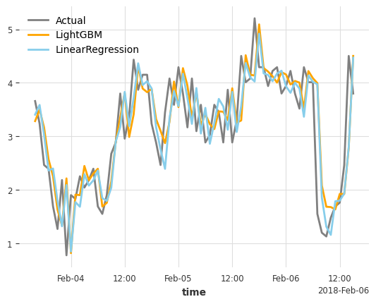

11.3 Covariates

So far we have used only the past values of a series to forecast its future values. However, often we also have data on other variables which can provide us information about our target variable. These are known as covariates. Making use of these variables can often improve the quality of our forecasts. Covariates can be divided into three groups:

Past covariates: These are variables whose values are only known up to the forecast time. For example, when forecasting electricity load, past weather measurements can be used as past covariates. Or when forecasting sales of ice-cream we can use GDP as a covariate.
Future covariates: These are variables whose future values are known in advance or can be reliably forecasted. The most import such variables are calendar information (day of week, holidays), pre-scheduled events, or weather forecasts. Future covariates allow models to account for upcoming changes that are known to the forecaster. We must be very careful to distinguish between past and future covariates. If we include about as a future covariates some variable whose values we would not reliably know at prediction time, we will end up with a model that may work very well on historical data but which would be of no use in making actual forecasts.
Time-invariant covariates: These variables remain constant throughout the series. They might include characteristics of the entity being forecasted, such as the capacity of a transformer or the demographic profile of a region. Such covariates become important only when we are trying to forecast multiple time series. For example you may be trying to forecast the sales of a dozen flavours of ice-cream. One approach would be to fit a dozen different models, one for each flavour. But since we expect some commonality across flavours, a better idea might be to build what is know as a global model in which we pool together data from all flavours, adding the flavour’s name and its characteristics as time-invariant covariates and then fit a single model which can simultaneously learns both common patterns and flavour-specific idiosyncracies.

In our examples the load variables are instances of past covariates, since it is unlikely that we’d know the future load at the time of predictions. We can include calendar characteristics such as month and hour of day as future covariates as both load and ambient temperatures depend on them.

Let’s create data series for these covariates:

# Create past covariates for load variables
load_cols = ['HUFL', 'HULL', 'MUFL', 'MULL', 'LUFL', 'LULL']

# Create past covariates from training data
past_covariates_train = TimeSeries.from_dataframe(
    train_df, 
    time_col='date', 
    value_cols=load_cols
)

# Create past covariates from test data
past_covariates_test = TimeSeries.from_dataframe(
    test_df, 
    time_col='date', 
    value_cols=load_cols
)

We don’t have to create the calendar covariates as darts has a built in feature to add them to the model. Let’s fit a LightGBM model that includes both kinds of covariates.

lgbm2_model = LightGBMModel(
    lags=L,
    lags_past_covariates=L,
    lags_future_covariates=(L,1),
    add_encoders={
        'datetime_attribute': {
            'future': ['month', 'day', 'hour']
        },
    })
# Fit the model
lgbm2_model.fit(ot_train,
                past_covariates=past_covariates_train)

[LightGBM] [Info] Auto-choosing col-wise multi-threading, the overhead of testing was 0.095053 seconds.
You can set `force_col_wise=true` to remove the overhead.
[LightGBM] [Info] Total Bins 74955
[LightGBM] [Info] Number of data points in the train set: 13888, number of used features: 483
[LightGBM] [Info] Start training from score 14.701914

LightGBMModel(lags=48, lags_past_covariates=48, lags_future_covariates=(48, 1), output_chunk_length=1, output_chunk_shift=0, add_encoders={'datetime_attribute': {'future': ['month', 'day', 'hour']}}, likelihood=None, quantiles=None, random_state=None, multi_models=True, use_static_covariates=True, categorical_past_covariates=None, categorical_future_covariates=None, categorical_static_covariates=None)

The code above creates and trains a LightGBM model that leverages both past and future covariates. Let’s examine each parameter in detail:

lags=L: This parameter sets the lookback window for the target variable (OT) to 48 hours, meaning the model will use the previous 48 hours of temperature data when making predictions.
lags_past_covariates=L: This sets the lookback window for past covariates to 48 hours as well, meaning the model will use the previous 48 hours of load variables when making predictions.
lags_future_covariates=(L,1): This tuple specifies the range of lags for future covariates, from L time steps in the past to 1 time step in the future. This allows the model to consider both historical and near-future calendar information.
add_encoders: This parameter adds uses a darts feature to add calendar variables as future covariates. Encoders are somewhat like scikit-learn’s column transformers, datatime_attribute can extract components from the time index. We add our attributes as future attributes since we would have the calendar available while making forecasts.

The model is then trained with fit() using two inputs:

ot_train: The target variable time series (transformer operating temperature)
past_covariates_train: The load variables we previously defined

The Darts framework automatically handles the alignment of these different time series, making it simple to incorporate multiple types of data in our forecasting model. By including calendar features, the model can learn seasonal patterns related to day, month, and hour, which are crucial in electricity load and temperature forecasting.

Let’s see how well we have done.

lgbm2_mse = lgbm2_model.backtest(ot_test, 
                            past_covariates=past_covariates_test,
                            forecast_horizon=1,
                            stride=1,
                            retrain=False,
                            metric=mse)
print(f"LightGBM with covariates model MSE: {lgbm2_mse:0.3f}")

LightGBM with covariates model MSE: 0.408

We see that the addition of covariates leads to a significant accuracy for our model.

11.4 Horizon

So far we have forecasted only one period ahead. A more challenging task is to make long-term forecasts. Suppose we want to forecast the transformer’s temperature profile for the next 96 hours. We have a number of ways to do this:

Recursive forecasts: Using data upto time \(t\), we use a one-period-ahead model forecast \(y_{t+1}\). Then we use treat this forecast as actually observed data and add it to our input series. We now use are one-period-ahead model with this augmented data to forecast \(y_{t+1}\) and so on. This method has the advantage of simplicity. However, in this approach there is a divergence between what the model was trained for (one-period-ahead forecasts) and what it is used for (multi-period forecasts). Such divergences may lead to poor performance.
Direct forecast: We fit a model to make the entire 96-hour ahead forecast. This poses a challenge if our regression model can produce only one prediction at a time. If we have to use such a model, we will have to fit 96 different models, one for each hour in the future. However, many regression models can produce a multivariate prediction, so direct forecasts are quite feasible.

Models in darts take a parameter output_chunk_length which determines what forecast horizon the model is fit on. Somewhat confusingly functions like predict take a parameter n which specifies the horizon for the forecast to be produced. What actually happens is that behind the scenes darts uses a direct forecast if n <= output_chunk_length and recursive forecast otherwise.

Let us use linear regression for our 96-hour forecast with calendar features as covariates. There are some minor changes from our earlier code: - We increase the lookback period to 720 to provide our models with more data. - We add a Scaler to our encoders. This normalizes our time series and is specially important for neural network models and does no harm for other models. We have left it out in our earlier code only for simplicity. - We add a stride parameter to backtest. This determines how much the backtest sliding window moves forward in each iteration. By making it equal to the horizon we make sure that the forecast windows we are testing our model over do not overlap.

from darts.models import LinearRegressionModel
from darts.dataprocessing.transformers import Scaler

# Set up a model for 24-hour forecasts
L=720
horizon = 96
lr_multi_model = LinearRegressionModel(
    lags=L,
    output_chunk_length=horizon,
    add_encoders={
        'datetime_attribute': {
            'future': ['month', 'day', 'hour', 'dayofweek']
        },
        'transformer': Scaler()
    }
)

# Fit the model
lr_multi_model.fit(ot_train)

# Evaluate using backtest
lr_multi_mse = lr_multi_model.backtest(
    ot_test,
    forecast_horizon=horizon,
    stride=horizon,
    retrain=False,
    metric=mse
)

print(f"Linear Regression {horizon}-hour forecast MSE: {lr_multi_mse:0.3f}")

Linear Regression 96-hour forecast MSE: 6.527

This time we compare the performance of this model with the model known as TiDE. TiDE (Time-series Dense Encoder) is a modern neural network architecture specifically designed for time series forecasting. It was developed by Google researchers and has shown strong performance on a variety of forecasting tasks. The model works as follows:

It uses a fully-connected neural network architecture with separate encoder and decoder components
The encoder processes historical data (input chunks) into a hidden state which the decoder takes as inputs generates forecasts (output chunks)
It handles multiple covariables through specialized embedding layers

The key hyperparameters that we will have to configure are:

input_chunk_length: The length of historical data used (our lookback window L)
output_chunk_length: The forecast horizon (96 hours in our case)
hidden_size: The dimensionality of hidden representations in the network (512)
num_encoder_layers/num_decoder_layers: The depth of the encoder/decoder networks (2 each)
decoder_output_dim: The dimension of the decoder output layer (32)
dropout: Regularization parameter to prevent overfitting (0.5)
use_layer_norm: Whether to use layer normalization to stabilize training

Darts implements the model using PyTorch Lightning. Parameters of the model constructor and the fit method allow us to control the training process. We illustrate this by seting the training rate and configuring early stopping. The hyperparameters are chosen to match the original TiDE paper.

from darts.models import TiDEModel
from pytorch_lightning.callbacks import EarlyStopping

# Define an early stopping callback which we will pass to the trainer
my_stopper = EarlyStopping(
    monitor="val_loss",     # Metric to monitor
    patience=5,             # How many epochs to wait to make sure
                            #  that validation error is not improving
    min_delta=0.05          # The minimum descrease in validation
                            #   error that would be considered an improvement
)

# Set up the TiDE model for 24-hour forecasts
tide_model = TiDEModel(
    input_chunk_length=L,
    output_chunk_length=horizon,
    optimizer_kwargs={"lr": 1e-3}, # Learning rate. Passed on to the optimizer
    num_encoder_layers=2,
    num_decoder_layers=2,
    decoder_output_dim=32,
    hidden_size=512,
    use_layer_norm=True,
    dropout=0.5,
    pl_trainer_kwargs={"callbacks": [my_stopper]}, #Callback, pass to trainer
    add_encoders={
        'datetime_attribute': {
            'past': ['month', 'day', 'hour', 'dayofweek'],
            'future': ['month', 'day', 'hour', 'dayofweek']
        },
        'transformer': Scaler()
    },
    random_state=110
)

# Create a validation set from the last 10% of training data
# A validation set is essential for early stopping to work                 
val_size = int(len(ot_train) * 0.2)
ot_val = ot_train[-val_size:]                               
ot_train_subset = ot_train[:-val_size]
                                                                            
past_covariates_val = past_covariates_train[-val_size:]
past_covariates_train_subset = past_covariates_train[:-val_size]
                                                                                
# Fit the model with early stopping using validation data                     
tide_model.fit(                                                                
    series=ot_train_subset,                 past_covariates=past_covariates_train_subset,           
    val_series=ot_val,
    val_past_covariates=past_covariates_val,          
    dataloader_kwargs = {'batch_size': 512}, #Passed to dataloader
    epochs=50,                    
)

Let’ now evaluate the model:

tide_mse = tide_model.backtest(
    ot_test,
    past_covariates=past_covariates_test,
    forecast_horizon=horizon,
    stride=horizon,
    retrain=False,
    metric=mse
)

print(f"TiDE {horizon}-hour forecast MSE: {tide_mse:0.3f}")

TiDE 96-hour forecast MSE: 8.005

After a very long computation the deep learning model actually fails to beat linear regression! In its defence we did not give it a very large dataset. Trying the problem with larger data and tuning the hyperparameters is left to you as an exercise.

11.5 Leave it to the machine

We have been fitting models taken as black-boxes from standard libraries using hyperparameter values that we have picked up from somewhere. Doesn’t it feel somewhat mechanical? Can’t we get machines to do this? Actually we can.

There are multiple ‘automatic machine learning’ frameworks available that automatically clean and transform data, fit a set of leading models using default hyperparameters or conduct a hyperparameter search and finally give you the best model. They can even create an ensemble of the best few models for you.

One such auomatic machine learning framework is AutoGluon https://auto.gluon.ai/ by Amazon. It has facilities for tabular, multimodal (image, text and tabular) and time series forecasting. We illustrate its use on our forecasting problem here.

We first import the library and create TimeSeriesDataFrame objects for our test and training datasets since that is the form in which the library expects its data.

from autogluon.timeseries import TimeSeriesDataFrame, TimeSeriesPredictor

train_data = TimeSeriesDataFrame.from_data_frame(
    train_df,
    id_column="ID",
    timestamp_column="date"
)

test_data = TimeSeriesDataFrame.from_data_frame(
    test_df,
    id_column="ID",
    timestamp_column="date"
)

Next we define a predictor

predictor = TimeSeriesPredictor(
    prediction_length=96,
    path="autogluon-etth1",
    target="OT",
    eval_metric="MSE",
)

We provie a forecast horizon, the path to the folder where all the fitted models and logs would be saved, the target time series and evaluation metric. Then we fit,

predictor.fit(
    train_data,
    presets="best_quality",
)

Fit will successively fit multiple models to the data and chose the best. All the models fit will be saved in the directory provided. The presets argument determines which models will be fit and allows the user to trade off between fitting time and quality. You can also specify a time limit to fit.

Once the model is fit we can evaluate it on the test dataset

print(predictor.leaderboard(test_data))

And you are done.

So what have we been doing all this while, when machines have already learnt to do machine learning for you? Do you need to read anything in this book apart from this section? Here’s what I think:

Automatic machine learning is a great way of getting routine experimentation out of the way.
Humans can then bring domain knowledge to bear in gathering, cleaning and organising data and making use of the recommendations of ML models.
Humans can then spend their time building bespoke solutions for problem that don’t fit neatly into standard models.
Humans can use their knowledge of existing models to come up with newer and better models and theoretical analyses to go with them.

11.6 What have we missed

As we said at the outset, this chapter only has presented some highlights of time series forecasting. There are many things left untouched.

We have not talked about the traditional, so-called ‘statistical’ models for time-series forecasting such as ARIMA and exponential smoothing. These models can be competitive with fancier machine learning techniques for smaller and simpler problems and are worth trying.

We have completely skipped over an older generation of neural network-based time-series models. Recurrent Neural Networks (RNNs), LSTM (Long Short-Term Memory) models and GRU (Gated Recurrent Unit) models represent a very-different approach from the sliding window approach discussed in this chapter. They can deal with sequence of arbitrary length. As they go through observations they update an internal ‘state’, which can be though of an internal summary of what they have seen so far. Then they produce forecasts as a function of the state. In these they are descendants of earlier state-space models. At present they have been overshadowed by the sliding window approach. But there is a lot of intuitive sense behind the state-space approach too and it may very well make a comeback.

This chapter illustrated only one deep learning model, TiDE. There are many of them: N-BEATS, N-HITS, TSMixer, PatchTST and many more. None of them is a clear winner in performance and none of them, in my opinion, represent a clear methodological advance. You must chose between them empricially. Most are implemented in darts and the Nixtla libraries.

All our examples were with univariate series. Many of these models can work with multivariate series too. The workflow remains essentially the same.

Finally, throught this chapter we have made forecasts in terms of a single number, what are known as point forecasts. But in many applications it is much more useful to forecast a probability distribution of possible values. Many of the libraries and models we have discussed do support such probabilistic forecasts in different forms.

Time series were our taste of sequence data. Our next chapter will look at the sequences that are arguably essential to our humanity—text—and how machine learning has conquered it.

11.7 References

11.7.1 Classical forecasting

Hyndman, R.J. and Athanasopoulos, G. Forecasting: Principles and Practice, 3rd ed. https://otexts.com/fpp3/

11.7.2 Machine learning models

Joseph, M. and Tackes, J. (2024). Modern Time Series Forecasting With Python.

11.7.3 Overview of the field

Makridakis, S., Spiliotis, E., & Assimakopoulos, V. (2022). ‘M5 accuracy competition: Results, findings, and conclusions.’ International Journal of Forecasting, 38(4), 1346-1364. https://doi.org/10.1016/j.ijforecast.2021.11.013

11.7.4 Transformer data source

Zhou, H., Zhang, S., Peng, J., Zhang, S., Li, J., Xiong, H., & Zhang, W. (2020). Informer: Beyond Efficient Transformer for Long Sequence Time-Series Forecasting. arXiv preprint arXiv:2012.07436.