from pathlib import Path
import requests

# We take the path where we want to save the data as a string
#   and construct a `Path` object out of it. This gives us
#   access to useful attributes and methods which we use below
local_path = Path('data/fhvhv_tripdata_2024-01.parquet')

# The URL for the data
url = 'https://d37ci6vzurychx.cloudfront.net/trip-data/fhvhv_tripdata_2024-01.parquet'

# the `exists` method of a path check if a file or director
#   exists at that location
if not local_path.exists():
        # the `parent` attribute of a path gives its parent
        #    i.e. the directory one level up
        # the `mkdir` method of a path creates a directory at that
        #    location,  with `exist_ok=True` you do not get an error
        #    if the directory already exists
        local_path.parent.mkdir(exist_ok=True)

        # requests.get fetches a resource from a URL (web path)
        #    it returns a response object, the `content` attribute
        #    of which contains the actual content.
        #    the `write_bytes` method of a path writes the provided
        #    bytes into a file at that location
local_path.write_bytes(requests.get(url).content)3 Regression, ML style
Note
This is an EARLY DRAFT.
The first supervised machine learning model we will look at is one you must already be familiar with as a student of economics: linear regression. A linear regression model used for predicting \(y\) values falls naturally into the supervised learning framework. Specifically, we have a dataset of \((x, y)\) pairs (where \(x\) denotes the explanatory variables and \(y\) denotes the outcome), and we specify a parameterized function for making predictions. In the standard linear regression case, the model is
\[ \hat{y}_i = x_i \beta, \]
where \(\hat{y}_i\) is our prediction for the \(i\)-th observation, \(x_i\) is a row vector of values of explanatory variables (also called features in ML parlance) for a given observation \(i\), and \(\beta\) is a column vector of parameters we wish to learn. In ordinary least squares (OLS), the loss function is \((y_i - \hat{y}_i)^2\), which measures how poorly our model predicts \(y_i\). Minimizing the average of these squared errors by setting up the normal equations
\[ X' \bigl(y - X\beta\bigr) = 0, \]
gives the well-known OLS solution. In econometrics, finding \(\beta\) that solves this equation is called fitting the model; in machine learning, this same process is called training. Once fitted, we can use the resulting \(\beta\) to make predictions, which ML practitioners refer to as inference. We typically assess goodness-of-fit via a metric such as \(R^2\).
All modern machine learning, including large language models (LLMs), follows this general framework: we have data (features plus a target), choose a parametric or nonparametric model, define a loss function, optimize model parameters, and then evaluate predictive accuracy. Although the architectures can become extremely complex and the number of parameters can skyrocket, the fundamental ideas remain consistent with linear regression. Indeed, an AI system that can eloquently discuss poetry is, in a conceptual sense, a direct descendant of the familiar regression paradigm—just with billions of parameters and trained on a vast corpus of human text. As the saying goes, “quantity has a quality all of its own.”
In our discussion here, you may notice that we have not mentioned some familiar statistical concepts from econometrics, such as the error term or confidence intervals for coefficients. Traditional machine learning places the main emphasis on prediction—how well the model generalizes to unseen data—rather than on inference about parameters (like whether a slope coefficient is statistically significant). When all you care about is good predictions, classical statistical inference is secondary, only goodness of fit matters.
However, economists instead often focus on causal inference—that is, understanding the effect of interventions in a system rather than merely forecasting or recognizing patterns in a given data generating process. While prediction does have a place in econometric practice, much of current empirical economics centers on questions of causality. In the later chapters of this book, we will see how machine learning–based prediction can become part of a broader causal inference strategy. For now, though, our focus is on introducing the predictive task and seeing how linear regression is implemented in Python’s ML ecosystem.
3.1 The dataset
Our illustrative example uses data on ride-hailing (“high-volume for-hire vehicle,” HVFHV) trips from the New York City Taxi and Limousine Commission (TLC). This data, which includes detailed trip records, is available on the TLC’s website in Parquet format. Parquet is an open data format designed to allow efficient access to the data for analysis tasks. Most data analysis frameworks and applications can read and write Parquet files.
We assume that you have downloaded the January 2024 data to a data folder in your working directory, stored as fhvhv_tripdata_2024-01.parquet. At the time of writing the URL for this data is https://d37ci6vzurychx.cloudfront.net/trip-data/fhvhv_tripdata_2024-01.parquet
The following Python snippet checks if the file exists and downloads it if not, also creating the data folder if it does not exist. When writing notebooks which would be run repeatedly it is a good practice to first check for the file’s existence before downloading it so as to avoid overloading the server hosting the file.
Here we are using the standard library pathlib module to handle the file and folder operations. For downloads we use the requests library, which while not part of the Python standard library has become the most commonly used library for interacting with Internet resources.
Our goal in this chapter is to build a regression model to predict the taxi fare from certain trip characteristics.
3.1.1 Loading the data
We start by importing necessary Python libraries:
import pandas as pd
import seaborn as sns
import numpy as np
from sklearn.compose import ColumnTransformer
from sklearn.preprocessing import OneHotEncoder, StandardScaler, OrdinalEncoder
from sklearn.pipeline import Pipeline
from sklearn.linear_model import SGDRegressor, LinearRegression
from sklearn.metrics import mean_squared_error, r2_score, mean_absolute_error
from sklearn.model_selection import train_test_split
We then read in the Parquet file, specifying a subset of columns via the columns parameter:
df = pd.read_parquet('data/fhvhv_tripdata_2024-01.parquet',
                     columns = ['hvfhs_license_num','request_datetime',
                                'trip_miles','trip_time','base_passenger_fare',
                                'driver_pay','PULocationID','DOLocationID'])
Because Parquet stores data by columns, specifying only the columns you need (e.g., trip_miles and base_passenger_fare) greatly speeds up data loading.
3.2 Dataset Fields
The full dataset includes many fields, but we will use only a few. For reference, here is the complete list of available columns:
| Field Name | Description |
|---|---|
hvfhs_license_num |
TLC license number of the HVFHS base/business |
dispatching_base_num |
TLC Base License Number of the dispatching base |
pickup_datetime |
Date and time of trip pick-up |
dropoff_datetime |
Date and time of trip drop-off |
PULocationID |
TLC Taxi Zone where trip began |
DOLocationID |
TLC Taxi Zone where trip ended |
originating_base_num |
Base number that received original trip request |
request_datetime |
Date/time of passenger pickup request |
on_scene_datetime |
Driver arrival time at pickup (Accessible Vehicles only) |
trip_miles |
Total passenger trip miles |
trip_time |
Total passenger trip time in seconds |
base_passenger_fare |
Base fare before tolls, tips, taxes, and fees |
tolls |
Total toll charges for trip |
bcf |
Black Car Fund amount collected |
sales_tax |
NYS sales tax amount collected |
congestion_surcharge |
NYS congestion surcharge collected |
airport_fee |
$2.50 fee for LaGuardia, Newark, and JFK airports |
tips |
Total passenger tips |
driver_pay |
Total driver pay (excluding tolls/tips, net of fees) |
shared_request_flag |
Passenger agreed to shared/pooled ride (Y/N) |
shared_match_flag |
Passenger shared vehicle with another booking (Y/N) |
access_a_ride_flag |
Trip administered for MTA (Y/N) |
wav_request_flag |
Wheelchair-accessible vehicle requested (Y/N) |
wav_match_flag |
Trip occurred in wheelchair-accessible vehicle (Y/N) |
The identity of the ride-share company can be found from the license number in the hvfhs_license_num column. It uses the following coding:
| License Number | Company |
|---|---|
| HV0002 | Juno |
| HV0003 | Uber |
| HV0004 | Via |
| HV0005 | Lyft |
In case you are interested in the actual geographical locations corresponding the the pickup and dropoff location ids, the TLC website provides files with the details.
3.3 Data preparation
3.3.1 Exploration
Before beginning any data modelling task it is essential to completely understand the process through which the data was generated and collected, the space, time and organizational units it corresponds to, the units used, any special values used to indicate missingness or other special conditions. Next one must spend some time developing a first-hand familiarity with the data, plotting and tabulating various combinations of variables and browsing through sample observations to get a sense of the patterns in the data.
All real-world data has errors. All real-world variables have ambiguities. At the outset our minds are full of unexamined assumptions about the data many of which may not be true. Without a prolonged period spent getting familiar with the data it is very likely that our entire analysis will have errors at its foundation.
Unfortunately, data exploration is a hands-on task that is hard to teach in a textbook format. It can be learnt through apprenticeship. It is even better learnt in the school of hard knocks. Be wary, be sceptical, test and test again. Having satisfied our conscience with these words of advice, we just carry out some basic checks and proceed with the minimal data preparation needed to illustrate fitting a regression model.
df.columnsIndex(['hvfhs_license_num', 'request_datetime', 'trip_miles', 'trip_time',
'base_passenger_fare', 'driver_pay', 'PULocationID', 'DOLocationID'],
dtype='object')df.shape(19663930, 8)df.describe()| request_datetime | trip_miles | trip_time | base_passenger_fare | driver_pay | PULocationID | DOLocationID | |
|---|---|---|---|---|---|---|---|
| count | 19663930 | 1.966393e+07 | 1.966393e+07 | 1.966393e+07 | 1.966393e+07 | 1.966393e+07 | 1.966393e+07 |
| mean | 2024-01-16 22:16:37.965603 | 4.838587e+00 | 1.110470e+03 | 2.395925e+01 | 1.826909e+01 | 1.391361e+02 | 1.424193e+02 |
| min | 2023-12-31 23:01:55 | 0.000000e+00 | 0.000000e+00 | -4.309000e+01 | -6.776000e+01 | 1.000000e+00 | 1.000000e+00 |
| 25% | 2024-01-09 14:57:44 | 1.493000e+00 | 5.710000e+02 | 1.163000e+01 | 8.210000e+00 | 7.500000e+01 | 7.600000e+01 |
| 50% | 2024-01-17 08:05:05.500000 | 2.830000e+00 | 9.120000e+02 | 1.800000e+01 | 1.357000e+01 | 1.400000e+02 | 1.420000e+02 |
| 75% | 2024-01-24 13:28:24.750000 | 5.990000e+00 | 1.430000e+03 | 2.880000e+01 | 2.283000e+01 | 2.110000e+02 | 2.170000e+02 |
| max | 2024-02-01 00:07:07 | 4.176200e+02 | 5.206000e+04 | 1.911160e+03 | 1.218170e+03 | 2.650000e+02 | 2.650000e+02 |
| std | NaN | 5.698662e+00 | 7.722219e+02 | 2.053657e+01 | 1.546117e+01 | 7.490267e+01 | 7.777903e+01 |
From these, we might notice that the minimum fare is negative in some rows and that some distances are zero. Such anomalies or errors are common in large-scale real-world datasets and must be dealt with before model training. We examine distributions:
df['base_passenger_fare'].hist()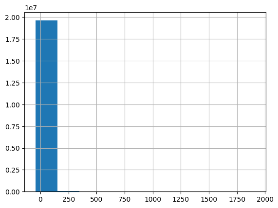
df['trip_miles'].hist()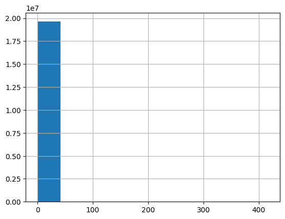
3.3.2 Cleaning
Based on the histograms and domain knowledge, we see that fares may contain negative outliers (e.g., erroneous entries or data processing glitches), and distances can be zero or extremely large. In this example, we apply simple filters:
- Keep trips where
trip_milesis between 1 and 20. - Keep trips where
base_passenger_fareis under $200.
These cutoffs are somewhat arbitrary but reflect a desire to capture typical trips. Realistically, any robust analysis would document and justify these choices.
df = df[(df['trip_miles']>=1)
            & (df['trip_miles']<=20)
            & (df['base_passenger_fare']<200)]
3.3.3 Feature creation
Feature engineering is the process of creating new features (or transforming existing ones) to enhance model performance. Despite the power of modern ML, including neural networks that can “learn” representations automatically, thoughtful feature engineering can still significantly improve accuracy and interpretability—especially for more transparent models like linear regression.
Here, we will:
- Extract the day of week (0 = Monday, …, 6 = Sunday): Demand and pricing patterns may be different on weekdays and weekends. Even among weekdays there may be patters. Maybe a rush to get away from office early on Fridays?
- Extract the hour of day (0–23): Demand for taxis certainly varies by hour of day. To the extent there is surge pricing, we need this variable to capture the demand effect.
- Create fare_per_mile as our new target variable, normalizing the fare by the trip distance: one natural reason for fare to differ is that longer trips will have higher fare. This a source of variation in fares which is expected and not very interesting. By making fare per mile our target variable, we eliminate this uninteresting variation.
df['request_day_of_week'] = df['request_datetime'].dt.dayofweek
df['request_hour_of_day'] = df['request_datetime'].dt.hour
df['fare_per_mile'] = df['base_passenger_fare']/df['trip_miles']
The .dt accessor is a pandas feature that provides access to datetime properties and methods when working with datetime-like series. It allows us to easily extract components like day of week or hour from datetime columns.
We now separate the dataset into features (\(X\)) and the target (\(y\)):
X = df[['hvfhs_license_num','trip_miles','trip_time',
        'request_day_of_week','request_hour_of_day','PULocationID','DOLocationID']]
y = df['fare_per_mile']
3.4 The train-test split
As we have seen in the previous chapter, we should keep aside a test set from the data which is not used in fitting the model so that it can later be used to estimate the model’s performance on new data. We again use scikit-learn’s test_train_split function for this:
X_train, X_test, y_train, y_test = train_test_split(X, y,
                                    test_size=0.2, random_state=100)
We allocate 20% of the data to the test set and set random_state=100 for reproducibility.
3.5 Preprocessing data
Unlike R’s lm() or Stata’s built-in regressions, scikit-learn requires explicit encoding of categorical variables. We typically rely on one-hot encoding to convert such variables into numeric format. One-hot encoding is nothing but the creation of dummy variables. If a categorical variable has \(m\) values, one-hot encoding generates \(m-1\) dummy variables to take its place.
Similarly, we often scale numerical features to have comparable ranges, which can substantially improve the optimization process for many algorithms.
Scikit-learn supports these and many more transformations through a common transformers API (not to be confused with the deep learning architecture called transformers). Each transformer is represented by a class which provides the following functions:
fit: to learn the parameters of the transformation from provided data. For exampleStandardScalarmay calculate the mean and standard deviations so that it can apply the transformation: \[x'_i = \frac{x_i - \bar x}{\text{sd}_x}\]transform: Once the parameters of the transformation have been learnt,transformtransforms the provided data according to those parameters. It is important that the data being transformed could be different from the data the parameters were learnt from.fit_transform: to learn parameters and carry out the transformation on the same data. The learnt parameteres are still retained in the transformer object and can be used to transform other data.
Let’s illustrate this with a concrete example using StandardScaler on the trip_time feature:
# Create a sample of trip times (in seconds)
trip_times = pd.Series([600, 1200, 900, 1800, 300], name='trip_time')

# Initialize and fit the scaler
scaler = StandardScaler()
scaler.fit(trip_times.values.reshape(-1, 1))

# The scaler has learned these parameters:
print("Mean of trip_time: {:.2f}".format(scaler.mean_[0]))
print("Standard deviation of trip_time: {:.2f}".format(scaler.scale_[0]))

# Transform the original data
scaled_times = scaler.transform(trip_times.values.reshape(-1, 1))
print("\nOriginal trip times:", trip_times.values)
print("Scaled trip times:", scaled_times.ravel())

# Now transform some new data using the same scaling parameters
new_trip_times = pd.Series([450, 2000, 750], name='trip_time')
new_scaled_times = scaler.transform(new_trip_times.values.reshape(-1, 1))
print("\nNew trip times:", new_trip_times.values)
print("New scaled times:", new_scaled_times.ravel())
Mean of trip_time: 960.00
Standard deviation of trip_time: 516.14
Original trip times: [ 600 1200 900 1800 300]
Scaled trip times: [-0.69748583 0.46499055 -0.11624764 1.62746694 -1.27872403]
New trip times: [ 450 2000 750]
New scaled times: [-0.98810493 2.01495907 -0.40686674]This example shows how StandardScaler first learns the mean and standard deviation from the data during fit(), then uses these parameters to transform the data to have zero mean and unit variance. The same scaler can then be used to transform new data using the same parameters.
Separation of fitting and transformation in the transformer API is important when we consider the train-test split. Because the test data has to be kept aside during the training process, any scaling we do had to be learnt from the training data. But then if the test data has to be fed into a model that was fitted to the scaled data, the same scaling has to be applied to the test data. Holding the scaling parameters in a transformer object makes this easy.
One-hot encoding works similarly.
Let’s see how OneHotEncoder works with categorical data, particularly with the handle_unknown='ignore' parameter:
# Create a sample of ride-share companies
companies = pd.Series(['Uber', 'Lyft', 'Via', 'Uber', 'Lyft'], name='company')

# Initialize and fit the encoder
encoder = OneHotEncoder(drop='first', handle_unknown='ignore')
encoder.fit(companies.values.reshape(-1, 1))

# The encoder has learned these categories:
print("Learned categories:", encoder.categories_[0])

# Transform the original data
encoded_companies = encoder.transform(companies.values.reshape(-1, 1))
print("\nOriginal companies:", companies.values)
print("Encoded companies:\n", encoded_companies)

# The output above shows a sparse matrix representation where:
# - (row, column) coordinates indicate where 1's occur
# - All other positions contain 0's
# - For example, (0, 0) means row 0, column 0 has value 1.0
# - This format saves memory by only storing non-zero values

# Now transform new data with an unknown category
new_companies = pd.Series(['Uber', 'Juno', 'Lyft'], name='company')
new_encoded = encoder.transform(new_companies.values.reshape(-1, 1))
print("\nNew companies:", new_companies.values)
print("New encoded (notice how 'Juno' is handled):\n", new_encoded)
Learned categories: ['Lyft' 'Uber' 'Via']
Original companies: ['Uber' 'Lyft' 'Via' 'Uber' 'Lyft']
Encoded companies:
<Compressed Sparse Row sparse matrix of dtype 'float64'
with 3 stored elements and shape (5, 2)>
Coords Values
(0, 0) 1.0
(2, 1) 1.0
(3, 0) 1.0
New companies: ['Uber' 'Juno' 'Lyft']
New encoded (notice how 'Juno' is handled):
<Compressed Sparse Row sparse matrix of dtype 'float64'
with 1 stored elements and shape (3, 2)>
Coords Values
(0, 0) 1.0The handle_unknown='ignore' parameter is crucial when dealing with categorical data that might contain new categories at prediction time. Without it, encountering an unknown category (like ‘Juno’ in our example) would raise an error. With handle_unknown='ignore', unknown categories are encoded as all zeros, allowing our model to gracefully handle new categories it hasn’t seen during training. Of course this is the right approach if unknown categories are likely to be rare. This would be the case if the number of categories is small relative to the size of the data.
3.5.1 Column transformers
At this point we could construct and use a transformer for each of our variables. We would have to gather together our numeric columns in one dataframe to feed to a StandardScalar and our categorical variables in another dataframe to feed to a OneHotEncoder. Then we would have to put the results back together. Thankfully, scikit-learn provides a ColumnTransformer class to take care of these details for us.
We first make separate lists of our numeric and categorical columns.
categorical_features = ['PULocationID','DOLocationID',
                        'hvfhs_license_num', 'request_day_of_week', 'request_hour_of_day']
numerical_features = ['trip_miles', 'trip_time']
Now a column transformer allows us to easily apply the the StandardScaler to each of the numeric column and OneHotEncoder to each of our categorical columns.
# Create and fit the column transformer
ct = ColumnTransformer([
    ('num', StandardScaler(), numerical_features),
    ('cat', OneHotEncoder(drop='first', handle_unknown='ignore'), categorical_features)
])

# Fit and transform the training data
X_train_transformed = ct.fit_transform(X_train)

# Transform test data using the fitted transformer
X_test_transformed = ct.transform(X_test)

# Show the shape of transformed data
print("Original training shape:", X_train.shape)
print("Transformed training shape:", X_train_transformed.shape)
Original training shape: (13616772, 7)
Transformed training shape: (13616772, 551)The increase in the number of columns is due to one-hot encoding of categorical variables. Each category (except one) in each categorical feature becomes a new column.
The ColumnTransformer takes a list of tuples, where each tuple has three elements:
- A name (like ‘num’ or ‘cat’) that identifies the transformer
- The transformer object itself (like StandardScaler or OneHotEncoder)
- The list of column names this transformer should be applied to
For example in ('num', StandardScaler(), numerical_features):
- ‘num’ is just a label we chose to identify this transformation
- StandardScaler() is the transformer that will standardize our numeric data
- numerical_features is our list containing ‘trip_miles’ and ‘trip_time’
Similarly, ('cat', OneHotEncoder(...), categorical_features) specifies how to handle our categorical columns.
Note that we use a single StandardScaler for all numerical features. The StandardScaler internally handles each feature independently, so there’s no need for separate scalers per feature. The same is true for OneHotEncoder.
3.6 Fitting the model
Just like the standardized interface for transformers, sci-kit learn has a set of classes with standard interface for different kind of machine learning models. Each of them has a fit function for fitting data and estimating parameters and a predict function for producing predicted values after estimation.
The class for linear regression is LinearRegressor. We can fit our model thus:
# Don't run this yet, we are going to do something cleverer

# Create and fit the model
model = LinearRegression()
model.fit(X_train_transformed, y_train)

# Make predictions
y_pred = model.predict(X_test_transformed)

# Print some basic metrics
print(f"R² Score: {r2_score(y_test, y_pred):.4f}")
3.7 Scikit-learn pipelines
Having seen how transformers and models work individually, we can now explore scikit-learn’s pipeline system which elegantly combines these components. A pipeline bundles multiple steps - like our ColumnTransformer for preprocessing and LinearRegression for modeling - into a single cohesive unit. This bundling offers several significant advantages over managing these steps separately.
First, pipelines enforce a clean separation between training and testing data. When preprocessing steps like scaling or encoding are performed outside a pipeline, there’s a risk of data leakage - where information from the test set inadvertently influences the training process. Pipelines automatically handle this separation by learning preprocessing parameters only from training data.
Another key benefit is reproducibility. All transformation parameters and model hyperparameters are stored together in the pipeline object. This makes it easier to save complete models, share them with colleagues, or deploy them in production environments. When you load a saved pipeline, you get back not just the trained model but also all the preprocessing steps with their learned parameters.
Pipelines also streamline the experimentation process. When trying different modeling approaches, you can easily swap out components while keeping the overall structure intact. For example, you might try different scalers (StandardScaler vs. RobustScaler) or different regression models (LinearRegression vs. Ridge) by changing just one line of code. This modularity makes it easier to systematically explore different modeling choices.
Furthermore, pipelines integrate seamlessly with scikit-learn’s more advanced model training and optimization tools, which we’ll explore in later chapters. This integration allows us to systematically improve our models while maintaining the clean organization that pipelines provide.
Here how to construct a pipeline to combine our preprocessing and estimation steps:
preprocessor = ColumnTransformer(
    transformers=[
        ('num', StandardScaler(), numerical_features),
        ('cat', OneHotEncoder(drop='first', handle_unknown='ignore'), categorical_features)
    ])

# Create the pipeline
pipeline = Pipeline([
    ('preprocessor', preprocessor),
    ('regressor', LinearRegression())
])
The Pipeline is constructed as a list of (name, transformer) tuples, where each name is a string identifier and each transformer is a scikit-learn transformer or estimator. In our case:
The first tuple
('preprocessor', preprocessor):- ‘preprocessor’ is the name we give this step
- preprocessor is our ColumnTransformer that handles both numeric and categorical features
The second tuple
('regressor', LinearRegression()):- ‘regressor’ is the name for our model step
- LinearRegression() is the actual model that will be fitted
When we call pipeline.fit(X_train, y_train), the steps are executed in order: first the preprocessor scales numeric features and one-hot encodes categorical features, then the transformed data is passed to the LinearRegression estimator for fitting via OLS. This approach helps prevent data leakage (where information from the test set could inadvertently influence the training process) and keeps code organized.
pipeline.fit(X_train, y_train)Pipeline(steps=[('preprocessor',
ColumnTransformer(transformers=[('num', StandardScaler(),
['trip_miles', 'trip_time']),
('cat',
OneHotEncoder(drop='first',
handle_unknown='ignore'),
['PULocationID',
'DOLocationID',
'hvfhs_license_num',
'request_day_of_week',
'request_hour_of_day'])])),
('regressor', LinearRegression())])In a Jupyter environment, please rerun this cell to show the HTML representation or trust the notebook. On GitHub, the HTML representation is unable to render, please try loading this page with nbviewer.org.
Pipeline(steps=[('preprocessor',
                 ColumnTransformer(transformers=[('num', StandardScaler(),
                                                  ['trip_miles', 'trip_time']),
                                                 ('cat',
                                                  OneHotEncoder(drop='first',
                                                                handle_unknown='ignore'),
                                                  ['PULocationID',
                                                   'DOLocationID',
                                                   'hvfhs_license_num',
                                                   'request_day_of_week',
                                                   'request_hour_of_day'])])),
('regressor', LinearRegression())])ColumnTransformer(transformers=[('num', StandardScaler(),
['trip_miles', 'trip_time']),
('cat',
OneHotEncoder(drop='first',
handle_unknown='ignore'),
['PULocationID', 'DOLocationID',
'hvfhs_license_num', 'request_day_of_week',
'request_hour_of_day'])])['trip_miles', 'trip_time']
StandardScaler()
['PULocationID', 'DOLocationID', 'hvfhs_license_num', 'request_day_of_week', 'request_hour_of_day']
OneHotEncoder(drop='first', handle_unknown='ignore')
LinearRegression()
3.8 Checking the overall quality of our fit
Once the pipeline is trained, we evaluate it on the held-out test set. We compute standard regression metrics such as Mean Squared Error (MSE), Root Mean Squared Error (RMSE), Mean Absolute Error (MAE), and \(R^2\). Each metric offers a different perspective on how well our model’s predictions match the observed data:
y_pred = pipeline.predict(X_test)
mse = mean_squared_error(y_test, y_pred)
rmse = np.sqrt(mse)
mae = mean_absolute_error(y_test, y_pred)
r2 = r2_score(y_test, y_pred)
print(f'Mean Squared Error: {mse:.4f}')
print(f'Root Mean Squared Error: {rmse:.4f}')
print(f'Mean Absolute Error: {mae:.4f}')
print(f'R² Score: {r2:.4f}')
Mean Squared Error: 5.1602
Root Mean Squared Error: 2.2716
Mean Absolute Error: 1.4254
R² Score: 0.4522A small MSE or MAE indicates that, on average, the predictions are close to the actual values. The RMSE is the square root of MSE and has the same units as the target variable, making it more interpretable. The \(R^2\) score (coefficient of determination) captures the fraction of variance in \(y\) explained by the model. An \(R^2\) near 1 indicates a strong fit, whereas a value near 0 suggests limited explanatory power.
Our model’s performance metrics (R² = 0.4522, RMSE = 2.2716, MAE = 1.4254), we can see that our linear regression model captures moderate but not strong predictive power for ride-share fares per mile. The R² value indicates that our model explains about 45% of the variance in per-mile fares, suggesting there’s still considerable unexplained variation in pricing. The RMSE of 2.27 and MAE of 1.43 indicate that our typical prediction errors are relatively large compared to the mean fare per mile, pointing to opportunities for model improvement.
Of course this is no reason to be disappointed. The linear regression model is the simplest model we could have used. With such a simple model feature engineering becomes very important. If we were carrying out this analysis for real, we would try to gather more domain knowledge about commuting in NYC and use that to create more effective features. But even that, or shifting to more complex models, would not guarantee success. There may be an inherent limit to how predictable some phenomena are.
In any case our result serves as a cautionary message about ‘big data’. Our dataset is certainly big, about 19 million observations. But that did not automatically lead to success in predicton.
3.9 Saving and reloading pipelines
Once we have a trained pipeline, we often want to save it for later use. This is particularly important in production environments where we want to use the same model consistently over time. Scikit-learn provides the joblib library for this purpose:
from joblib import dump, load

# Save the pipeline to a file
dump(pipeline, 'ride_share_model.joblib')

# Later, we can load it back
loaded_pipeline = load('ride_share_model.joblib')

# The loaded pipeline works exactly like the original
y_pred_new = loaded_pipeline.predict(X_test)
print(f"R² Score with loaded model: {r2_score(y_test, y_pred_new):.4f}")
R² Score with loaded model: 0.4522The saved pipeline includes:
- All preprocessing steps with their learned parameters (means, standard deviations, etc.)
- The trained model coefficients
- The structure of the pipeline itself
This means we can use the loaded pipeline to make predictions on new data without having to recreate or retrain any components. This is particularly useful when:
- Deploying models to production systems
- Sharing models with colleagues
- Comparing model versions over time
- Creating model backups
3.10 Conclusion
Choose a model, fit, predict, check performance. This is the standard routine of machine learning practice. In this chapter we saw how to carry out these tasks in scikit-learn. The next few chapters will introduce different machine learning model classes and libraries and we will see how to carry out the same steps in those contexts.
3.11 Exercise
Carry out as many of the indicated next steps in the chapter by:
- Looking at other analyses of New York Taxi data (this is a very popular example dataset)
- Obtaining the actual locations corresponding to the location ids, finding location ids with extreme values, and trying to understand what might have generated those values
- We have used the base fare in our analysis. Was that a good idea? What happens if you add tolls, surcharges etc?
- We did not use the ride-sharing flag. Does excluding shared rides make any differences?