5  Optimization

Note

This is an EARLY DRAFT.

Optimization is a central part of machine learning. As we saw at the outset, our goal in machine learning is to find a predictor that minimizes risk and we often go about this by minimizing functions such as empirical risk.

We avoided directly dealing with optimization problems in the last two chapters for two different reasons. In the case of ordinary least squares regression, the first order conditions for optimality takes the form of the normal equation

$${\mathbf{X}}^{\mathrm{\top }}(\mathbf{y}-\mathbf{X}\mathit{\beta })=0$$

which is a linear equation in $\beta$. For moderately-sized datasets forming the matrix $X$ and solving this linear equation is a reasonable way of finding the optimal $\beta$.

In the case of decision trees we do not optimize a global objective function. The fitting of decision trees tries to maximize homogeneity on a per-leaf basis in the hope that it will lead to a good tree overall.

However, as we move forward in machine learning we will have to solve optimization problems where neither of these approaches work. It will then become important to make use of algorithms that through a series of numerical calculations find approximate optimal points of functions. In this chapter we look at a very important class of these algorithms — algorithms based around the idea of gradient descent.

5.1 Some theory

In optimization theory, we often encounter the concepts of local and global minima. A point $x^{\ast }$ is a local minimum of a function $f$ if there exists some neighborhood around $x^{\ast }$ where $f(x^{\ast })$ is less than or equal to $f(x)$ for all points $x$ in that neighborhood. In other words, $f(x\ast )$ is the smallest value of the function in some small region around $x^{\ast }$. A global minimum, on the other hand, is a point where $f(x^{\ast })$ is less than or equal to $f(x)$ for all possible $x$ in the domain of $f$. Every global minimum is also a local minimum, but the reverse is not necessarily true.

For differentiable functions, we can characterize these minima using first-order conditions. In one dimension, a necessary condition for $x^{\ast }$ to be a local minimum is that the derivative equals zero at that point: $f^{\prime }(x^{\ast })=0$. This makes intuitive sense: if the derivative were positive, we could decrease f by moving left; if negative, by moving right. In multiple dimensions, this generalizes to requiring that all partial derivatives equal zero, or equivalently, that the gradient vector $\mathrm{\nabla }f(x^{\ast })=0$. These points where the gradient vanishes are called stationary points.

The gradient $\mathrm{\nabla }f$ at any point x is a vector of partial derivatives $[\partial f/\partial x_1,\dots ,\partial f/\partial x_n]$. A fundamental property of the gradient is that it points in the direction of steepest ascent - the direction in which f increases most rapidly. Consequently, $-\mathrm{\nabla }f$ points in the direction of steepest descent, which explains why gradient-based optimization algorithms typically move in the negative gradient direction. The magnitude of the gradient $\parallel \mathrm{\nabla }f\parallel$ indicates how steep the function is at that point.

For convex functions, which can be thought of as functions whose graph lies above any tangent plane, the optimization landscape is particularly nice. In a convex function, any local minimum is guaranteed to also be a global minimum. Moreover, if the function is strictly convex, this minimum is unique.

However, many objective functions in machine learning, particularly in deep learning, are not convex. Neural networks, for instance, typically have highly non-convex loss surfaces with many local minima. The loss surface might also contain saddle points (where the gradient is zero but the point is neither a minimum nor a maximum) and plateaus (regions where the gradient is very close to zero). This complex landscape makes optimization challenging and explains why sophisticated optimization algorithms have been developed beyond simple gradient descent.

The presence of multiple local minima in non-convex problems raises an important practical question: if we can’t guarantee finding the global minimum, what should we aim for? In machine learning, it turns out that many local minima are often “good enough” in terms of prediction performance. Recent research even suggests that in very high-dimensional problems, most local minima tend to have similar values, making the distinction between local and global minima less critical than one might expect.

5.2 Gradient descent

Gradient descent is an iterative optimization algorithm that follows a simple yet powerful principle: repeatedly take small steps in the direction that reduces the function’s value most quickly. The algorithm starts at an initial point and follows these steps: first, it calculates the gradient (derivative) of the function at the current position; second, it moves in the opposite direction of this gradient by a small amount (the learning rate); finally, it repeats these steps until reaching a point where the gradient is effectively zero or after a predetermined number of iterations. This process is analogous to finding the bottom of a valley by always walking downhill in the steepest direction available.

5.2.1 The Gradient Descent update rule

Suppose we are trying to minimize the function $f(\mathbf{x})$. Let ${\mathbf{x}}^{(t)}$ denote the value of $\mathbf{x}$ iteration $t$. The gradient descent update is:

$${\mathbf{x}}^{(t+1)}={\mathbf{x}}^{(t)}-\alpha \mathrm{\nabla }f({\mathbf{x}}^{(t)}),$$ where $\alpha$ is the learning rate (or step size). Choosing $\alpha$ is crucial:

• If $\alpha$ is too large, the algorithm might skip over a minimum or diverge.
• If $\alpha$ is too small, convergence can be very slow.

In practice, finding a good learning rate can be done through trial and error or using adaptive strategies. The universal concept, though, is that each update step is a small movement down the slope of $f$.

5.2.2 Example: Minimizing $ f(x) = x^2 $

To illustrate how gradient descent works, consider the one-dimensional function: $$f(x)=x^2.$$ We know from basic calculus that its minimum is at $ x^* = 0 $. Let us see how gradient descent iteratively converges to this solution.

5.2.2.1 Deriving the Gradient and Update

Here, the gradient (which reduces to a derivative in 1D) is: $$f^{\prime }(x)=2x.$$ The gradient descent update for a current estimate $ x^{(t)} $ is: $$x^{(t+1)}=x^{(t)}-\alpha \cdot 2x^{(t)}=x^{(t)}(1-2\alpha ).$$ If $|1-2\alpha |<1$, the sequence $\{x^{(t)}\}$ converges to 0. If $1-2\alpha \ge 1$ or $1-2\alpha \le -1$, we will fail to converge (or even diverge).

5.2.2.2 Numerical illustration

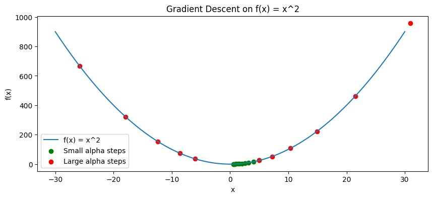
Below we code the gradient descent algorithm for $ f(x) = x^2 $ and explore the effect of different learning rates:

import numpy as np
import matplotlib.pyplot as plt

def f(x):
    return x**2

def f_prime(x):
    return 2*x

# Parameters
alpha_small = 0.1   
alpha_large = 1.1   
num_iterations = 10
x_initial = 5.0

def gradient_descent(x0, alpha, iterations):
    x_vals = [x0]
    for i in range(iterations):
        grad = f_prime(x_vals[-1])
        x_next = x_vals[-1] - alpha * grad
        x_vals.append(x_next)
    return x_vals

# With a smaller learning rate
x_vals_small = gradient_descent(x_initial, alpha_small, num_iterations)

# With a larger learning rate
x_vals_large = gradient_descent(x_initial, alpha_large, num_iterations)

print("Learning rate (alpha) = 0.1:")
print([f"{x:0.2f}" for x in x_vals_small])

print("\nLearning rate (alpha) = 1.0:")
print([f"{x:0.2f}" for x in x_vals_large])

# Plotting
x_plot = np.linspace(-30, 30, 100)
y_plot = f(x_plot)

plt.figure(figsize=(10,4))
plt.plot(x_plot, y_plot, label="f(x) = x^2")
plt.scatter(x_vals_small, [f(x) for x in x_vals_small], 
            color='green', label="Small alpha steps")
plt.scatter(x_vals_large, [f(x) for x in x_vals_large],
            color='red', label="Large alpha steps")
plt.title("Gradient Descent on f(x) = x^2")
plt.xlabel("x")
plt.ylabel("f(x)")
plt.legend()
plt.show()

Learning rate (alpha) = 0.1:
['5.00', '4.00', '3.20', '2.56', '2.05', '1.64', '1.31', '1.05', '0.84', '0.67', '0.54']

Learning rate (alpha) = 1.0:
['5.00', '-6.00', '7.20', '-8.64', '10.37', '-12.44', '14.93', '-17.92', '21.50', '-25.80', '30.96']

• When $\alpha =0.1$, the sequence converges toward 0, the minimum.
  
• When $\alpha =1.0$, it diverges (the updates overshoot).

This example reveals a fundamental truth about gradient descent in higher-dimensional problems as well:

• Too large a learning rate can cause your updates to bounce away from a minimum.
• Too small a learning rate can make convergence painstakingly slow.

In practical machine learning, one often uses learning rate schedules (where $\alpha$ decreases over time) or more sophisticated methods with adaptive step sizes. These refinements help ensure that early in training, the algorithm takes larger steps for quick progress, and later, smaller steps for fine-tuning.

5.3 Stochastic Gradient Descent (SGD)

For large-scale machine learning problems, computing the exact gradient for a loss function over a massive dataset can be computationally expensive. Stochastic Gradient Descent (SGD) addresses this by estimating the gradient using only a small subset of the data at each iteration.

The effectiveness of SGD in machine learning stems from the structure of our objective functions. Consider empirical risk minimization (ERM), where we minimize:

$$\frac{1}{n}\sum _{i=1}^n\ell (\theta ;x_i,y_i)$$

This is an average over all observations. By the law of large numbers, we can estimate this average using a small random sample of observations. While this introduces noise into our gradient estimates, the noise is unbiased - its expected value equals the true gradient. The learning rate plays a crucial role here: smaller learning rates reduce the impact of noisy updates but slow convergence, while larger rates allow faster progress but may amplify the effects of noise. This trade-off is why learning rate schedules, which gradually decrease α over time, are often effective in practice.

5.3.1 Core Concepts and Terminology

1. Batch: In standard “batch” gradient descent, the entire dataset is used to compute the gradient before each update.
   
2. Minibatch: A subset of the dataset (e.g., 32, 64, or 128 samples). Minibatch gradient descent balances computational efficiency and smoothing of gradient estimates.
   
3. Epoch: One complete pass over the entire dataset. If you have $N$ data points and the minibatch size is $B$, then $\lceil N/B\rceil$ updates make up one epoch.
   
4. Iterations (or Steps): Each gradient update is one iteration. After enough iterations, you typically hope to see convergence to a satisfactory solution.

5.3.2 The SGD Update Rule

Let $\mathcal{L}(\mathit{\theta })$ be the loss over the entire dataset of size $N$: $$\mathcal{L}(\mathit{\theta })=\frac{1}{N}\sum _{i=1}^N\ell (\mathit{\theta };{\mathbf{x}}_i,y_i).$$

• Batch Gradient Descent uses $${\mathit{\theta }}^{(t+1)}={\mathit{\theta }}^{(t)}-\alpha \mathrm{\nabla }\mathcal{L}({\mathit{\theta }}^{(t)}).$$

• Stochastic (or Minibatch) Gradient Descent uses a small batch $B_t$: $${\mathit{\theta }}^{(t+1)}={\mathit{\theta }}^{(t)}-\alpha \frac{1}{|B_t|}\sum _{j\in B_t}\mathrm{\nabla }\ell ({\mathit{\theta }}^{(t)};{\mathbf{x}}_j,y_j).$$

Here, $\alpha$ is again the learning rate, but in practice, we often let $\alpha$ decay over time (e.g., ${\alpha }_t={\alpha }_0/(1+kt)$) because the noisy gradient estimates can make the algorithm oscillate near a minimum.

For linear regression scikit-learn provides a model class SGDRegressor which fits the model using SGD instead of solving the normal equation. If you try it on a large dataset you’ll find that it runs much faster and has a predictive accuracy not much worse than fitting the model using LinearRegression model class which uses the normal equations.

SGD is indispensable for fitting models such as neural network where there are no closed-form solutions to the optimization problem. However the simple version of the SGD we have discussed so far have some limitation and many advanced variants have been invented.

5.4 Problems with SGD in the multidimensional case

A fundamental challenge with gradient descent emerges when optimizing functions where different parameters have substantially different scales of impact on the loss function. These scenarios are ubiquitous in machine learning: neural network parameters often have widely varying effects on the output. In this case a learning rate which is so large that it causes oscillations along one dimensional may be so small along another dimension that it delays convergence inordinately.

To illustrate this problem concretely, consider minimizing a simple quadratic function:

$$f(x,y)=\frac{1}{2}{x}^2+\frac{70}{2}{y}^2$$

This function has several instructive properties:

• It has a unique global minimum at (0,0)
• The y-coordinate has 70 times more influence on the loss than x
• The loss surface forms a narrow valley, steep in y but shallow in x

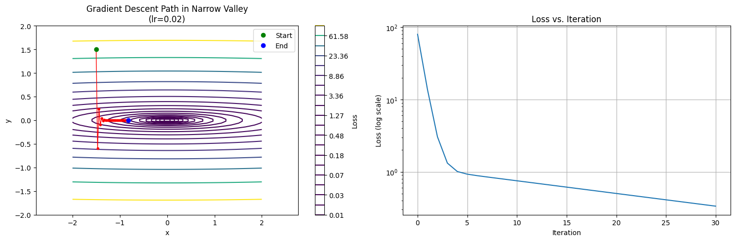
The following code demonstrates how gradient descent behaves in this challenging landscape. Pay particular attention to the ratio of movements in the y versus x directions, which reveals the algorithm’s inefficient zigzagging behavior.

import numpy as np
import matplotlib.pyplot as plt

# Create a loss function that forms a narrow valley
# f(x,y) = ax²/2 + by²/2 where a << b creates a narrow valley
def loss_function(x, y, a=1, b=70):  
    return a * x**2/2 + b * y**2/2

def gradient(x, y, a=1, b=70):  
    return np.array([a * x, b * y])

# Set up the grid for plotting
x = np.linspace(-2, 2, 100)
y = np.linspace(-2, 2, 100)
X, Y = np.meshgrid(x, y)
Z = loss_function(X, Y)

# Initialize parameters for gradient descent
learning_rate = 0.02  
num_iterations = 30
start_point = np.array([-1.5, 1.5])

# Run gradient descent 
def gradient_descent():
    points = [start_point]
    current = start_point.copy()
    
    for _ in range(num_iterations):
        grad = gradient(current[0], current[1])
        update = learning_rate * grad
        current = current - update
        points.append(current.copy())
    
    return np.array(points)

# Run the optimization
trajectory = gradient_descent()

# Create visualization
plt.figure(figsize=(15, 5))

# Plot 1: Contour plot with trajectory
plt.subplot(121)
plt.contour(X, Y, Z, levels=np.logspace(-2, 2, 20))
plt.colorbar(label='Loss')
plt.plot(trajectory[:, 0], trajectory[:, 1], 'ro-', linewidth=1, markersize=3)
plt.plot(trajectory[0, 0], trajectory[0, 1], 'go', label='Start')
plt.plot(trajectory[-1, 0], trajectory[-1, 1], 'bo', label='End')
plt.xlabel('x')
plt.ylabel('y')
plt.title('Gradient Descent Path in Narrow Valley\n(lr=0.02)')
plt.legend()
plt.axis('equal')

# Plot 2: Loss over iterations
plt.subplot(122)
losses = [loss_function(p[0], p[1]) for p in trajectory]
plt.semilogy(range(len(losses)), losses)
plt.xlabel('Iteration')
plt.ylabel('Loss (log scale)')
plt.title('Loss vs. Iteration')
plt.grid(True)

plt.tight_layout()
plt.show()

# Calculate and print some statistics
print(f"Starting loss: {losses[0]:.3f}")
print(f"Final loss: {losses[-1]:.3f}")
print(f"Reduction in loss: {(1 - losses[-1]/losses[0])*100:.1f}%")

# Show the zigzag behavior by printing distances moved in x and y
x_movements = np.abs(np.diff(trajectory[:, 0]))
y_movements = np.abs(np.diff(trajectory[:, 1]))
print(f"\nAverage movement per step:")
print(f"X-direction: {np.mean(x_movements):.3e}")
print(f"Y-direction: {np.mean(y_movements):.3e}")
print(f"Y/X movement ratio: {np.mean(y_movements)/np.mean(x_movements):.1f}")

# Print first few updates to show the zigzagging pattern
print("\nFirst few updates:")
for i in range(min(5, len(trajectory)-1)):
    dx = trajectory[i+1,0] - trajectory[i,0]
    dy = trajectory[i+1,1] - trajectory[i,1]
    print(f"Step {i+1}: dx={dx:.3e}, dy={dy:.3e}, |dy/dx|={abs(dy/dx):.1f}")

Starting loss: 79.875
Final loss: 0.335
Reduction in loss: 99.6%

Average movement per step:
X-direction: 2.273e-02
Y-direction: 1.167e-01
Y/X movement ratio: 5.1

First few updates:
Step 1: dx=3.000e-02, dy=-2.100e+00, |dy/dx|=70.0
Step 2: dx=2.940e-02, dy=8.400e-01, |dy/dx|=28.6
Step 3: dx=2.881e-02, dy=-3.360e-01, |dy/dx|=11.7
Step 4: dx=2.824e-02, dy=1.344e-01, |dy/dx|=4.8
Step 5: dx=2.767e-02, dy=-5.376e-02, |dy/dx|=1.9

The visualization and numerical results reveal several key insights about gradient descent’s behavior in poorly conditioned optimization problems:

1. Zigzagging Pattern: The trajectory shows dramatic oscillations, particularly evident in the step-by-step analysis:
   • Initial step: $|\mathrm{\Delta }y/\mathrm{\Delta }x|=70.0$, reflecting the raw gradient ratio
   • By step 5: $|\mathrm{\Delta }y/\mathrm{\Delta }x|=1.9$, showing reduced but still uneven progress
   • Average ratio: 5.1 over all steps
2. Loss Reduction Phases: $$\begin{array}{rl}\text{Starting loss}& =79.875\\ \text{Final loss}& =0.335\\ \text{Reduction}& =99.6\mathrm{\%}\end{array}$$ While the overall reduction is impressive, the loss curve shows:
   • Rapid initial descent (dominated by y-correction)
   • Followed by much slower progress (limited by x-direction)
3. Learning Rate Dilemma: The choice of learning rate ($\alpha =0.02$) represents a compromise:
   • Must be small enough to avoid overshooting in the sensitive y-direction ($\alpha <\frac{2}{70}$ for stability)
   • But this makes progress in the x-direction very slow ($\alpha \ll \frac{2}{1}$)

This example generalizes to higher dimensions: when different parameters have vastly different scales of influence on the loss, gradient descent is forced to use a learning rate appropriate for the most sensitive direction. This creates inefficient trajectories that zigzag through narrow valleys rather than moving directly toward the minimum.

Understanding this fundamental limitation of gradient descent helps explain why more sophisticated optimization methods are often necessary for complex machine learning models.

5.5 Adam Optimizer

Plain SGD requires one global learning rate and can be sensitive to gradient noise. Adam (Adaptive Moment Estimation) enhances SGD by keeping per-parameter running averages of both the gradient and its square (or “second moment”). This helps in:

• Adaptive Step Sizes: Each parameter has its own effective learning rate, shrinking updates in directions where gradients have been large or volatile.
  
• Smoothing Out Noise: By taking moving averages, the algorithm reduces the randomness of individual minibatch updates.

Adam often converges faster and more robustly than vanilla SGD, especially in high-dimensional or complex models.

5.5.1 Intuitive Motivation

Imagine walking on uneven terrain in the dark:

• With plain SGD, you choose one step size and take equally sized steps in whatever direction the gradient points.
  
• Adam effectively “feels out” the terrain, adjusting its step size based on how bumpy or steep each dimension is. Parameters that experience large gradient swings receive smaller updates; others can move more freely.

5.5.2 The Adam Update Rule

At iteration $ t $, let ${\mathit{\theta }}_t$ be your parameters and ${\mathbf{g}}_t={\mathrm{\nabla }}_{\mathit{\theta }}\mathcal{L}({\mathit{\theta }}_t)$ be the gradient. Adam maintains two exponentially decaying averages:

1. First moment (${\mathbf{m}}_t$), akin to momentum: $${\mathbf{m}}_t={\beta }_1{\mathbf{m}}_{t-1}+(1-{\beta }_1){\mathbf{g}}_t.$$
2. Second moment (${\mathbf{v}}_t$), capturing the magnitude/variance: $${\mathbf{v}}_t={\beta }_2{\mathbf{v}}_{t-1}+(1-{\beta }_2){\mathbf{g}}_t^2.$$

Typical defaults: ${\beta }_1=0.9$, ${\beta }_2=0.999$. Early in training, these running averages are small, so Adam applies bias corrections:

$${\hat{\mathbf{m}}}_t=\frac{{\mathbf{m}}_t}{1-{\beta }_1^t},{\hat{\mathbf{v}}}_t=\frac{{\mathbf{v}}_t}{1-{\beta }_2^t}.$$

The final parameter update is:

$${\mathit{\theta }}_{t+1}={\mathit{\theta }}_t-\alpha \frac{{\hat{\mathbf{m}}}_t}{\sqrt{{\hat{\mathbf{v}}}_t}+\epsilon },$$ where $\alpha$ is the global learning rate (often ${10}^{-3}$) and $\epsilon \approx {10}^{-8}$ avoids division by zero.

5.5.3 Practical Benefits

1. Less Hyperparameter Tuning: Adam is typically more forgiving of suboptimal $\alpha$ choices.
   
2. Faster Convergence: In many real-world tasks, Adam converges more quickly than plain SGD.
   
3. Stability: The second-moment estimate helps curb wild oscillations.

5.5.4 Final Thoughts on Adam

Adam is the go-to optimization method for a wide range of machine learning models. Its adaptive per-parameter step size often yields faster progress on complex objectives, making it an especially popular choice in deep learning. The principles behind Adam—taking an average of first and second moments of gradients—carry over to many advanced optimizers that refine or extend these ideas.

5.6 Automatic Differentiation

While we’ve discussed various optimization algorithms that use gradients, we haven’t yet addressed how to compute these gradients efficiently. For simple functions, we can derive gradients analytically, but for complex models like neural networks, this becomes impractical. Automatic differentiation (autodiff) solves this problem by automatically computing exact derivatives through a computational graph representation of functions.

5.6.1 Motivation

Consider computing gradients for a neural network with millions of parameters. Three approaches are possible:

1. Manual differentiation: Deriving and coding gradients by hand. Error-prone and impractical for complex models.
2. Numerical differentiation: Using finite differences like $(f(x+h)-f(x))/h$. Simple but numerically unstable and computationally expensive.
3. Automatic differentiation: Applying the chain rule systematically through the computation graph. Exact, efficient, and automatic.

5.6.2 How Autodiff Works

Automatic differentiation breaks down complex functions into elementary operations (addition, multiplication, sin, exp, etc.) and applies the chain rule systematically. For example, consider:

$$f(x)=\sin (x^2)$$

Autodiff would: 1. Break this into $y=x^2$ and $f=\sin (y)$ 2. Track both the value and derivative at each step 3. Apply the chain rule: $f^{\prime }(x)=\cos (y)\cdot \frac{dy}{dx}=\cos (x^2)\cdot 2x$

5.6.3 Illustration

All neural network frameworks have support for automatic differentiation. For now, we will illustrate the idea using the autograd library which can automatically differentiate Python functions, including those which use NumPy.

You will have to install autograd in your environment by running

pip install autograd

in a terminal or

!pip install autograd

in a Jupyter notebook cell.

In the following code we define a function to calculate $f(x)=x^2+\sin (3x)$ and use autograd to automatically derive its gradient.

import autograd.numpy as np  # Wraps NumPy functions
from autograd import grad    # The automatic differentiation function
import matplotlib.pyplot as plt

# Define a complex function
def f(x):
    return x**2 + np.sin(3*x)

# Get its derivative automatically
df = grad(f)

# Create points for plotting
x = np.linspace(-2, 2, 100)
y = f(x)
dy = np.array([df(x_i) for x_i in x])  # Compute derivative at each point

# Visualize the function and its derivative
plt.figure(figsize=(10, 5))
plt.plot(x, y, label='f(x) = x² + sin(3x)')
plt.plot(x, dy, label="f'(x) = 2x + 3cos(3x)")
plt.grid(True)
plt.legend()
plt.title('Function and its Automatically Computed Derivative')
plt.show()

# Verify at a specific point
x0 = 1.0
print(f"At x = {x0}:")
print(f"f'(x) = {df(x0):.4f}")
print(f"Analytical value = {2*x0 + 3*np.cos(3*x0):.4f}")

5.6.4 Multiple Variables and Gradients

Autodiff naturally extends to multiple variables. Here’s an example computing partial derivatives:

from autograd import grad

def f(x):  # x will be an array [x1, x2]
    return x[0]**2 * np.exp(-x[1])

# Partial derivatives
grad_x1 = grad(f, 0)  # with respect to first argument
grad_x2 = grad(f, 1)  # with respect to second argument

x = np.array([1.0, 2.0])
print(f"∂f/∂x₁ at {x} = {grad_x1(x):.4f}")
print(f"∂f/∂x₂ at {x} = {grad_x2(x):.4f}")

5.6.5 Key Benefits

1. Exactness: Unlike numerical differentiation, autodiff computes exact derivatives (up to floating-point precision).
2. Efficiency: The computational cost is typically only a small constant factor times the cost of computing the original function.
3. Composability: Can handle arbitrary compositions of differentiable operations.
4. Automatic: No need to manually derive or implement gradient formulas.

These properties make autodiff essential for modern machine learning, where we need to efficiently compute gradients of complex loss functions with respect to thousands or millions of parameters.

5.7 Concluding Thoughts

Optimization algorithms in machine learning and largely revolve around the core principle of following the gradient—the local direction of steepest descent. From simple gradient descent to SGD to Adam, each method refines how we choose the step size or how we incorporate past gradient information to navigate the loss landscape more effectively.

For newcomers, the most important concepts to grasp are: - Why the gradient determines the local best direction to move when seeking a minimum.
- How the step size (learning rate) affects convergence behavior and must be tuned or adapted.
- Why stochastic or adaptive methods (SGD, Adam) are practical for large-scale or noisy problems.

By understanding these, one gains a powerful lens through which to tackle a wide range of machine learning and economic optimization tasks.