In the previous chapter, we introduced regression—focusing on linear regression as a foundational supervised learning model. While our models in the previous chapter only included terms which were linear in the explanatory variables, you would know from your econometrics courses that linear regression models can also include nonlinear transformations of variables, as well as interactions among variables. In fact, introducing such terms may be essential for getting a good fit. However, for regression models we have to use our judgement to decide which nonlinearities and interactions to introduce, since we know that if we introduce too many, we face the danger of overfitting. While there are extensions of linear regression such as the lasso or ridge regression which tackle this problem, in this chapter we look at an alternative class of models, decision trees, that can learn nonlinearities and interactions from the data itself.
Decision trees can be used both for regression (numeric outcome) and classification (categorical outcome) tasks. However, in this chapter we will look at an classification examples so that we can also introduce ideas and concepts common to all classification approaches.
4.1 What is a decision tree?
Here’s a simple decision tree for predicting if someone has a high income (>50K) based on age and education years:
                     Root
                Age <= 30?
                   /    \
                  /      \
               Yes        No
              /            \
        Predict:        Education>=12?
        Income<=50K        /        \
                        /          \
                      No           Yes
                      |             |
                   Predict:        Predict:
                   Income<=50K     Income>50K
Given the age and education data for an individual this tree can be used to make prediction for that individual’s income class.
If Age ≤ 30: Predicts Income ≤ 50K
If Age > 30 and Education < 12: Predicts Income ≤ 50K
If Age > 30 and Education ≥ 12: Predicts Income > 50K
Decision trees like the one above consist of two kinds of nodes:
Internal nodes are decision points that split the data (like “Education >= 12?”). We shall only consider trees where each internal node looks at a single feature (explanatory variable) and has exactly two edges going out of it.
Leaf nodes are the terminal nodes that make predictions (like “Income <= 50K”). Each node predicts a single value: either a class in a classification problem or a predicted value in a regression problem.
If we draw a diagram with age on the \(x\)-axis and education on the \(y\)-axis then the internal nodes of the tree split the space into rectangular regions with boundaries parallel to the axes.
The “Age <= 30” node creates a vertical line at Age = 30
The “Education >= 12” creates a horizontal line at Education = 12 in the right-hand region created by the previous split
A deeper tree would break up a space into a larger set of regions. Within a given region the tree predicts a given value for the outcome.
This structure makes decision trees interpretable but also reveals their limitations: they can only create boundaries parallel to the axes, resulting in “boxy” decision regions. Axis-aligned rectangles in fancier terms. This is why they sometimes need many splits to approximate diagonal or curved boundaries.
4.2 Learning decision trees from data
4.2.1 Growing trees
We could try to apply the ERM paradigm to decision trees by trying to find the tree that minimizes empirical risk corresponding to some loss function among all possible trees. However this is computationally impractical. Instead, decision tree libraries try to find a good (i.e. low empirical risk) tree through an incremental process.
We begin the tree-growing procedure with a tree that is a single leaf node which is also the root. So at this point the tree has no branches at all. For any \(x\) we just predict the most common value of \(y\).
Then we start growing the tree by splitting of leaf nodes. For every leaf node we look at all possible variables and all possible split point for that variables. So we consider splits like “Age<50”, “Age<55”, “Education<12”, “Education<15” etc. We evaluate each split by seeing how it improves the ‘purity’, i.e. homogeneity of the two newly created leaf nodes relative to the homogeneity of the leaf node being split. This is because in any decision tree we make the same predictions for all \(x\) values that reach a given leaf node. So if we take our sample as indicative of the data distribution we would want all observations ending up in a given leaf to have the same \(y\) value as far as possible, so that when we use the most common value of \(y\) in a give leaf as our prediction we make as few misclassification errors as possible. We choose the best possible split according to this purity criterion, and then split the leaf.
We keep introducing splits in this manner and continue growing the tree until a stopping criterion is met. The stopping criteria may take the form of limits specified by the user on tree depth or size. Even if no such limits are specified, the tree-growing procedure stops either when each leaf contains a single observation or when no further splits improve purity.
4.2.1.1 Measuring Purity
To implement the algorithm above we need a measure of numerical measure of purity or homogeneity. Two measures of impurity in common use are:
Gini Impurity: \[
\text{Gini} = 1 - \sum_{c} p_c^2
\] where \(c\) represents each class (e.g., ≤50K and >50K in our income example) and \(p_c\) is the proportion of samples belonging to class \(c\) in the node.
Entropy: \[
\text{Entropy} = -\sum_{c} p_c \log p_c
\] with the same meaning for \(c\) and \(p_c\). For example, if a node has 70 samples of class ≤50K and 30 samples of class >50K, then \(p_{≤50K} = 0.7\) and \(p_{>50K} = 0.3\).
Both these measures take on the value 0 when all observations belong to the same class (with the convention that \(0\log 0=0)\) and take on positive values when the proportion in both classes is positive. There is no strong theoretical or empirical basis to choose one of these over the other.
4.2.2 Controlling Tree Growth
To prevent overfitting, we can control tree growth by specifying additional conditions to stop the splitting of tree nodes. The most important of these are:
Maximum depth: How many levels deep the tree can grow. Greater the permissible depth, greater is the number of trees that can be fit. This provides flexibility but at the same time increases the possibility of overfitting. This is the same approximation vs estimation error tradeoff that we have seen earlier.
Minimum number of samples per leaf: Restricting this prevents the tree growing algorithm from splitting leaves excessively to fit every peculiarity of the training sample.
4.2.3 Cost-Complexity Pruning
Cost-complexity pruning (also known as weakest link pruning) provides an alternative to restricting tree growth by setting a maximum depth or a minimum number of samples per leaf. Rather than limiting the tree’s development upfront (which risks missing useful splits), this method first grows a large, highly detailed tree and then prunes it back. The pruning process creates a sequence of progressively smaller subtrees, each one “optimal” for a given level of complexity.
To balance accuracy against size, define the cost-complexity measure for a subtree \(T\) as \[
R_\alpha(T) = R(T) + \alpha \, |T|,
\] where \(R(T)\) is the misclassification rate (or other error measure), \(|T|\) is the number of leaf nodes, and \(\alpha\) is a penalty parameter that increases the importance of tree size. As \(\alpha\) rises, subtrees with many leaves become more expensive, forcing the pruning procedure to remove them unless they significantly reduce error. At one extreme (\(\alpha = 0\)), the full tree remains; at the other (\(\alpha \to \infty\)), pruning continues until only a single node remains.
The pruning algorithm systematically identifies, for each \(\alpha\), the subtree \(T^*\) that minimizes \(R_\alpha(T)\). We as the users of the algorithm must provide the \(\alpha\) value to be used. We shall see below how we can use the data-driven method of cross-validation to make this choice.
The penalty term \(|T|\) introduces us to regularization, a fundamental technique in machine learning. Regularization works by adding a model complexity penalty to the loss function we want to minimize. This creates a crucial tradeoff: the model must balance minimizing training loss against keeping its complexity in check. While this helps prevent overfitting (since complex models are more prone to overfit), it comes with a tradeoff. By penalizing complexity, which isn’t part of our true objective, we potentially sacrifice some model accuracy. The parameter \(\alpha\) lets us control this tradeoff - higher values favor simpler models while lower values allow more complexity. Later, we’ll explore how to use data to guide our choice of \(\alpha\).
4.3 The Adult Income Dataset
Let us now see how to work with decision trees in scikit-learn. We will use the Adult dataset from the UCI Machine Learning Repository—often called the “Census Income” dataset. This dataset has over 32,000 observations in a typical train split, and more if combined with the test portion, making it large enough for realistic experimentation. The goal is to predict whether an individual’s income is >50K or <=50K based on demographic and employment features.
Key features include:
age (numeric)
education (categorical)
marital-status (categorical)
occupation (categorical)
hours-per-week (numeric)
… plus several others
Target: income (binary), which is either >50K or <=50K.
We will:
Load the dataset
Clean missing or unknown values
Convert categorical fields to numeric encodings
Split into train/test
Fit a decision tree classifier
Evaluate results
Discuss overfitting, pruning, and hyperparameter tuning via cross-validation
Note: We focus on classification here. One could also use decision trees for regression tasks (e.g., continuous income), but we leave that for a later demonstration or an exercise.
4.3.1 Loading and Preparing the Data
The Adult dataset is available on UCI Machine Learning Repository and can also be fetched via tools like fetch_openml in scikit-learn. Here, we’ll demonstrate the approach via fetch_openml for convenience.
import pandas as pdimport numpy as npimport seaborn as snsimport matplotlib.pyplot as pltfrom sklearn.datasets import fetch_openmlfrom sklearn.model_selection import train_test_split# Fetch the Adult dataset from OpenMLadult = fetch_openml(name='adult', version=2, as_frame=True)df = adult.frame # This is a pandas DataFrame# Inspect the DataFrameprint(df.shape)df.head()
(48842, 15)
age
workclass
fnlwgt
education
education-num
marital-status
occupation
relationship
race
sex
capital-gain
capital-loss
hours-per-week
native-country
class
0
25
Private
226802
11th
7
Never-married
Machine-op-inspct
Own-child
Black
Male
0
0
40
United-States
<=50K
1
38
Private
89814
HS-grad
9
Married-civ-spouse
Farming-fishing
Husband
White
Male
0
0
50
United-States
<=50K
2
28
Local-gov
336951
Assoc-acdm
12
Married-civ-spouse
Protective-serv
Husband
White
Male
0
0
40
United-States
>50K
3
44
Private
160323
Some-college
10
Married-civ-spouse
Machine-op-inspct
Husband
Black
Male
7688
0
40
United-States
>50K
4
18
NaN
103497
Some-college
10
Never-married
NaN
Own-child
White
Female
0
0
30
United-States
<=50K
4.3.2 Basic Cleaning
Some rows have ? in certain columns indicating missing data. Let’s filter those out for simplicity. In a more thorough analysis, you might impute or handle missingness carefully.
# Remove rows with '?' in certain columnsfor col in ['workclass', 'occupation', 'native-country']: df = df[df[col] !='?']# Now rename the target column for claritydf.rename(columns={'class': 'income'}, inplace=True)
4.3.3 Feature and Target Split
X = df.drop(columns='income')y = df['income']
4.3.4 Train-Test Split
As always, let’s hold out a separate test set for final evaluation:
Note: Setting stratify=y ensures that the split preserves the overall proportion of >50K vs. <=50K in both the training and test sets, which can be important if the classes are imbalanced.
4.3.5 Dealing with Categorical Features
Decision trees can directly handle categorical variables in theory, but scikit-learn’s DecisionTreeClassifier requires numeric arrays. Thus, we use one-hot encoding (creating dummy variables):
The argumet remainder="passthrough" specifies that all columns not listed explicitly should be passed through unchanged. The force_int_remainder_cols is to suppress an unncessary warning. verbose_feature_names controls whether the transformer name is prepended to the generated column names. We can set this to True to prevent name clashes. We don’t expect clashes, so we set it to False.
4.3.6 Training a Decision Tree Classifier
Let’s now create a pipeline that first transforms the data (via the ColumnTransformer) and then fits a DecisionTreeClassifier. This approach keeps the entire process (encoding + model) together and avoids data leakage.
from sklearn.pipeline import Pipelinefrom sklearn.tree import DecisionTreeClassifiertree_pipeline = Pipeline([ ('preprocessor', preprocessor), ('clf', DecisionTreeClassifier( max_depth =4, criterion='gini', random_state=42 ))])# Fit the pipeline on training datatree_pipeline.fit(X_train, y_train)
In a Jupyter environment, please rerun this cell to show the HTML representation or trust the notebook. On GitHub, the HTML representation is unable to render, please try loading this page with nbviewer.org.
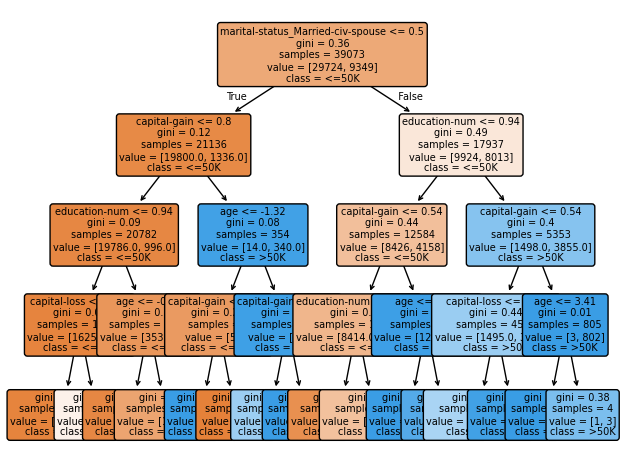
We arbitrarily set the maximum depth of the tree to 4 and chose the Gini impurity measure. Later in the chapter we shall see how to make these decisions in a data-guided manner.
4.3.7 Examining tree characteristics
We can query the depth and number of leaves directly from the fitted model.
print(f"Tree Depth: {tree_pipeline.named_steps['clf'].get_depth()}")print(f"Number of Leaves: {tree_pipeline.named_steps['clf'].get_n_leaves()}")
Tree Depth: 4
Number of Leaves: 16
The fitted model also provides feature importance scores which show how much each feature contributes to the tree’s decisions:
Each score ranges from 0 to 1, with all scores summing to 1
Higher scores indicate features used more often in important splits
The importance is calculated based on how much each feature’s splits improve the Gini impurity
We only show features with >1% importance to focus on the most influential variables
For example, if ‘age’ has a high importance score, it means splits on age tend to create purer subgroups and appear frequently in the tree’s important decisions.
The following code prints out features with greater than 1% importance.
# Get feature names:feature_names = tree_pipeline['preprocessor'].get_feature_names_out()# Create sorted feature importancesimportances = tree_pipeline['clf'].feature_importances_feature_importance =list(zip(feature_names, importances))feature_importance.sort(key=lambda x: x[1], reverse=True)print("\nFeature Importances (sorted):")for feature, importance in feature_importance:if importance >0.01: # Only show features with >1% importanceprint(f"{feature}: {importance:.3f}")
While lists of variable importance like this are useful in understanding what a tree is doing, one must guard against assigning any causal significance to these numbers.
For example, if ‘education’ appears high in feature importance, this does not imply that increasing education levels would cause higher incomes. The importance score merely reflects education’s predictive power in the current data generating process.
In fact, we need to be cautious even when interpreting importance score as a measure of a variable’s predictive power. There may very well be other trees which make equally good predictions but give importance to a different set of variables.
Therefore, strictly speaking, the importance numbers like the ones above are only a summary of a given tree. Reading anything more into them is a risky exercise.
4.3.8 Visualizing the tree
We can visualize our trained decision tree using scikit-learn’s tree plotting functionality:
from sklearn.tree import plot_treeimport matplotlib.pyplot as plt# Plot the tree plot_tree( tree_pipeline.named_steps['clf'], feature_names=feature_names, class_names=['<=50K', '>50K'], filled=True, rounded=True, fontsize=7, # Larger font size precision=2# Fewer decimal places in numbers)# Adjust layout to prevent text cutoffplt.tight_layout()plt.show()
4.4 Evaluating Performance
4.4.1 Accuracy and the confusion matrix
When evaluating classification models, especially in economic and policy contexts, we need to consider multiple performance metrics because different types of errors may have different costs.
The most basic performance measure is the accuracy — the proportion of test observations whose class is correctly predicted by the tree.
from sklearn.metrics import (accuracy_score, classification_report, roc_curve, auc)import matplotlib.pyplot as plt# Get predictionsy_pred = tree_pipeline.predict(X_test)# Basic accuracyacc = accuracy_score(y_test, y_pred)print(f"Test Accuracy: {acc:.4f}")
Test Accuracy: 0.8409
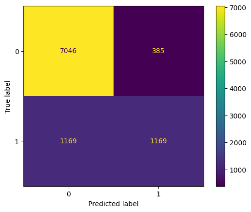
However, in many applications all misclassification errors are not equal. In our case classifying a low-income person as high-income may have completely different consequences from classifying a high-income person as low-income. A more detailed picture of the misclassification errors is presented by the confusion matrix.
from sklearn.metrics import ConfusionMatrixDisplayConfusionMatrixDisplay.from_predictions(y_test, y_pred)
The entry in row \(i\) and column \(j\) of the confusion matrix shows the number of observations actually in class \(i\) which were predicted to be in class \(j\). This lets us view at a glance the frequency of the different classes in the test sample as well as where misclassification errors occur.
The classification report provides another view of the misclassification errors.
In this report, for each class we are provided the following metrics:
Precision: When the model predicts this class, what fraction of times is it right? We want this to be high especially when false positives are expensive.
Recall: Of all actual cases in this class, what proportion were correctly predicted to belong to this class? We want this to be high especially when false negatives are expensive.
F1-score: Harmonic mean of precision and recall.
Support: The number of samples actually in this class.
In addition, the following aggregate metrics are provided:
Macro avg: Simple average of per-class metrics.
Weighted avg: Average of per-class metrics weighted by class support.
Accuracy: Overall correct predictions / total predictions
We see that our tree does much better in predicting the class “<=50K” than in predicting the class “>50K”. This is a common predicament when one class is underrepresented in the sample. We would have missed out on this if we had only looked at the overall accuracy.
4.4.2 ROC and AUC
Decision trees can provide probability estimates for each class, not just binary predictions. For each leaf node, the tree calculates the proportion of training samples in each class. When making predictions, instead of just returning the majority class, we can get these probabilities using predict_proba().
For example, if a leaf node has 70 samples with income ≤50K and 30 with income >50K, it will predict: - P(income ≤50K) = 0.7 - P(income >50K) = 0.3
To convert these probabilities into class labels, we need a threshold (default is 0.5). This creates an important tradeoff between the following two desirable characteristics:
Sensitivity (True Positive Rate): The proportion of actual positive cases (>50K) that are correctly identified
Specificity (True Negative Rate): The proportion of actual negative cases (≤50K) that are correctly identified
Lowering the threshold (e.g., to 0.3) makes the model more likely to predict >50K, increasing sensitivity but decreasing specificity. Raising it has the opposite effect. The choice depends on the relative costs of false positives versus false negatives in your application.
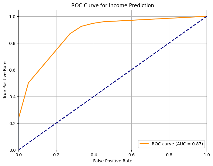
The Receiver Operating Characteristic (ROC) curve and Area Under the Curve (AUC) evaluates classifier performance across different probability thresholds. The ROC curve plots the True Positive Rate (sensitivity) against the False Positive Rate (1-specificity) at various classification thresholds. The more ‘outward’ the ROC curve, the better is our classifier, since for each value of specificity it has higher sensitivity. AUC is the area under this curve and provides a numerical summary of how ‘outward’ it is.
The ROC curve helps us understand: - How well the model distinguishes between classes - The tradeoff between true positives and false positives - Model performance at different classification thresholds
The AUC (Area Under the ROC Curve) ranges from 0 to 1: - AUC = 1.0: Perfect classification - AUC = 0.5: Random guessing (diagonal line) - AUC > 0.5: Better than random - Higher AUC indicates better model discrimination
In our case, an AUC of around 0.8 suggests the model has good discriminative ability between high and low income classes, though there’s still room for improvement.
4.5 Handling Class Imbalance
Suppose we cared as much about accuracy in prediction for both classes even though their proportions are very different in the data. One solution is to give greater weight to the underrepresented class when calculating purity of leaf nodes. In the example below we fit another tree to the data, this time passing the argument class_weight='balanced' to the DecisionTreeClassifier which causes it to weigh each class by the inverse of its frequency.
# Example with balanced class weightsbalanced_tree = Pipeline([ ('preprocessor', preprocessor), ('clf', DecisionTreeClassifier( class_weight='balanced', max_depth =4, random_state=42 ))])balanced_tree.fit(X_train, y_train)y_pred_balanced = balanced_tree.predict(X_test)print("Classification Report with Balanced Weights:")print(classification_report(y_test, y_pred_balanced))
If we compare this with the previous accuracy report, we see that we have achieved some improvement of the f1 score of the “>50K” class, though at a cost of the f1 score of the other class.
4.6 Hyperparameter Tuning with Cross-Validation
In machine learning, we distinguish between two types of model parameters:
Parameters: Values learned from the training data during model fitting
For decision trees, these include:
The specific feature used at each split node
The threshold values for each split
The predicted class in each leaf node
These are determined automatically by the learning algorithm
Hyperparameters: Configuration settings we choose before training
For decision trees, these include:
max_depth: Maximum depth of the tree
min_samples_leaf: Minimum samples required in a leaf
criterion: The splitting criterion (gini or entropy)
These control the model’s complexity and learning behavior
Must be set before training begins
While parameters are learned from data to minimize prediction error, hyperparameters are chosen to control the learning process itself. Poor hyperparameter choices can lead to underfitting (too simple) or overfitting (too complex) models.
We can systematically find good hyperparameter values (e.g., max_depth, min_samples_leaf) by using cross-validation (CV) on the training set.
Remember how we split our data into training and test sets? Cross-validation takes this idea further by creating multiple training-validation splits within the training data. Instead of a single validation set, we:
Divide the training data into \(K\) equal parts (called “folds”)
Train \(K\) different models, each using \(K-1\) folds for training and \(1\) fold for validation
Average the \(K\) validation scores to get a more robust estimate of model performance
This allows us to use the entire training data for both training and validation. Moreover, since the validation scores are sampled over all the folds, we can do with a smaller validation set sizes since the averaging should smooth out the sampling variations. helps avoid the luck (or bad luck) of a single validation split and gives us a better idea of how well our model will generalize. For example, with \(K=5\):
4.6.1 Grid Search vs Random Search
When tuning hyperparameters, we have two main strategies:
Grid Search (GridSearchCV in scikit-learn):
Tries every combination of specified parameter values
Random Search (RandomizedSearchCV in scikit-learn):
Randomly samples parameter combinations
Better for many parameters or continuous ranges
Often finds good values faster than grid search
Can specify number of iterations to control computation time
We illustrate below with a random search:
from sklearn.model_selection import RandomizedSearchCVfrom scipy.stats import randint, uniform# Define parameter distributionsparam_distributions = {'clf__max_depth': randint(3, 20), # Random integers between 3 and 20'clf__min_samples_leaf': randint(1, 20), # Random integers between 1 and 20'clf__ccp_alpha': uniform(0, 0.05) # Random floats between 0 and 0.05}# Initialize random searchrandom_search = RandomizedSearchCV( estimator=tree_pipeline, param_distributions=param_distributions, n_iter=50, # Number of parameter settings sampled cv=5, # 5-fold cross-validation scoring='accuracy', n_jobs=-1, # use all available CPU cores verbose=1, random_state=42# for reproducibility)# Fit random searchrandom_search.fit(X_train, y_train)print("Best Parameters:", random_search.best_params_)print("Best CV Accuracy:", random_search.best_score_)# Print all tried parameters sorted by scoreresults = pd.DataFrame(random_search.cv_results_)results = results.sort_values('rank_test_score')print("\nTop 5 Parameter Combinations:")for i inrange(5):print(f"\nRank {i+1}:")print(f"Parameters: {results.iloc[i]['params']}")print(f"Mean CV Score: {results.iloc[i]['mean_test_score']:.4f}")
Fitting 5 folds for each of 50 candidates, totalling 250 fits
After random search completes, the best estimator is fitted to the entire training dataset (without leaving out a validation fold) and is available in random_search.best_estimator_. Tts parameters are available in random_search.best_params_.
4.6.2 Final Model Evaluation on Test Set
After finding the best hyperparameters, we evaluate on the held-out test set to get an unbiased estimate of performance:
best_model = random_search.best_estimator_y_pred_optimized = best_model.predict(X_test)acc_optimized = accuracy_score(y_test, y_pred_optimized)print(f"Test Accuracy with Best Params: {acc_optimized:.4f}")print("\nClassification Report:")print(classification_report(y_test, y_pred_optimized))
Test Accuracy with Best Params: 0.8566

Classification Report:
              precision    recall  f1-score   support

       <=50K       0.88      0.95      0.91      7431
        >50K       0.77      0.57      0.66      2338

    accuracy                           0.86      9769
   macro avg       0.82      0.76      0.78      9769
weighted avg       0.85      0.86      0.85      9769
We see that the best estimator found through cross-validations do somewhat better than the arbitrarily chosen hyperparameters that we had used at the beginning.
4.7 Conclusion
The Adult dataset example we worked with is a binary classification problem: we have two classes (<=50K, >50K). In other tasks—say classifying a paper into “Reject”, “Revise” and “Accept”—we may have a larger number of outcome classes. Everything we have done above for the two-class case applies with commonsensical changes to this multiclass case as well. Decision trees can also be used for regression tasks. In scikit-learn we use DecisionTreeRegressor instead of DecisionTreeClassifier.
Because decision trees are highly flexible, they tend to suffer from high variance. In the next chapter, we will see how to use collections (ensembles) of trees rather than a single tree to address this limitation.
4.8 12. Exercises
Data Exploration: Download the Adult dataset directly from the UCI repository and replicate the analysis. Compare results with the fetch_openml approach.
Pruning vs. Depth Constraints:
Try setting different values of max_depth (e.g., 3, 5, 10) without pruning.
Also experiment with ccp_alpha for cost-complexity pruning (see scikit-learn docs).
Compare how these hyperparameters affect training accuracy vs. test accuracy.
Threshold Tuning: Use predict_proba to get predicted probabilities of income >50K. Plot the precision-recall curve and see how different classification thresholds affect the trade-off between precision and recall.
Regression Tree: Convert the “hours-per-week” column (or capital-gain) into a numeric target and try a regression tree approach. Examine MSE or R² on a hold-out set.
Feature Importance: In scikit-learn, DecisionTreeClassifier.feature_importances_ gives a measure of each feature’s importance. Print or plot these to see which features the tree relies on most. Are they in line with what you would expect from economic reasoning?
By exploring these exercises, you will deepen your understanding of how decision trees capture complex relationships, how to manage overfitting, and how to measure performance in line with specific economic or business objectives.
Source Code
::: {.callout-note}This is an **EARLY DRAFT**.:::# Decision TreesIn the previous chapter, we introduced **regression**—focusing on linear regression as a foundational supervised learning model. While our models in the previous chapter only included terms which were linear in the explanatory variables, you would know from your econometrics courses that linear regression models can also include nonlinear transformations of variables, as well as interactions among variables. In fact, introducing such terms may be essential for getting a good fit. However, for regression models we have to use our judgement to decide which nonlinearities and interactions to introduce, since we know that if we introduce too many, we face the danger of overfitting. While there are extensions of linear regression such as the lasso or ridge regression which tackle this problem, in this chapter we look at an alternative class of models, decision trees, that can learn nonlinearities and interactions from the data itself.Decision trees can be used both for **regression** (numeric outcome) and **classification** (categorical outcome) tasks. However, in this chapter we will look at an classification examples so that we can also introduce ideas and concepts common to all classification approaches.## What is a decision tree?Here's a simple decision tree for predicting if someone has a high income (>50K) based on age and education years:``` Root Age <= 30? / \ / \ Yes No / \ Predict: Education>=12? Income<=50K / \ / \ No Yes | | Predict: Predict: Income<=50K Income>50K```Given the age and education data for an individual this tree can be used to make prediction for that individual's income class.1. If Age ≤ 30: Predicts Income ≤ 50K2. If Age > 30 and Education < 12: Predicts Income ≤ 50K 3. If Age > 30 and Education ≥ 12: Predicts Income > 50KDecision trees like the one above consist of two kinds of nodes: - **Internal nodes** are decision points that split the data (like "Education >= 12?"). We shall only consider trees where each internal node looks at a single feature (explanatory variable) and has exactly two edges going out of it. - **Leaf nodes** are the terminal nodes that make predictions (like "Income <= 50K"). Each node predicts a single value: either a class in a classification problem or a predicted value in a regression problem.If we draw a diagram with age on the $x$-axis and education on the $y$-axis then the internal nodes of the tree split the space into rectangular regions with boundaries parallel to the axes. - The "Age <= 30" node creates a vertical line at Age = 30 - The "Education >= 12" creates a horizontal line at Education = 12 in the right-hand region created by the previous splitA deeper tree would break up a space into a larger set of regions. Within a given region the tree predicts a given value for the outcome.This structure makes decision trees interpretable but also reveals their limitations: they can only create boundaries parallel to the axes, resulting in "boxy" decision regions. **Axis-aligned rectangles** in fancier terms. This is why they sometimes need many splits to approximate diagonal or curved boundaries.## Learning decision trees from data### Growing treesWe could try to apply the ERM paradigm to decision trees by trying to find the tree that minimizes empirical risk corresponding to some loss function among all possible trees. However this is computationally impractical. Instead, decision tree libraries try to find a good (i.e. low empirical risk) tree through an incremental process.We begin the tree-growing procedure with a tree that is a single leaf node which is also the root. So at this point the tree has no branches at all. For any $x$ we just predict the most common value of $y$.Then we start growing the tree by splitting of leaf nodes. For every leaf node we look at all possible variables and all possible split point for that variables. So we consider splits like "Age<50", "Age<55", "Education<12", "Education<15" etc. We evaluate each split by seeing how it improves the ‘purity’, i.e. homogeneity of the two newly created leaf nodes relative to the homogeneity of the leaf node being split. This is because in any decision tree we make the same predictions for all $x$ values that reach a given leaf node. So if we take our sample as indicative of the data distribution we would want all observations ending up in a given leaf to have the same $y$ value as far as possible, so that when we use the most common value of $y$ in a give leaf as our prediction we make as few misclassification errors as possible. We choose the best possible split according to this purity criterion, and then split the leaf.We keep introducing splits in this manner and continue growing the tree until a stopping criterion is met. The stopping criteria may take the form of limits specified by the user on tree depth or size. Even if no such limits are specified, the tree-growing procedure stops either when each leaf contains a single observation or when no further splits improve purity.#### Measuring PurityTo implement the algorithm above we need a measure of numerical measure of purity or homogeneity. Two measures of impurity in common use are: **Gini Impurity**: $$ \text{Gini} = 1 - \sum_{c} p_c^2 $$ where $c$ represents each class (e.g., ≤50K and >50K in our income example) and $p_c$ is the proportion of samples belonging to class $c$ in the node. **Entropy**: $$ \text{Entropy} = -\sum_{c} p_c \log p_c $$ with the same meaning for $c$ and $p_c$. For example, if a node has 70 samples of class ≤50K and 30 samples of class >50K, then $p_{≤50K} = 0.7$ and $p_{>50K} = 0.3$.Both these measures take on the value 0 when all observations belong to the same class (with the convention that $0\log 0=0)$ and take on positive values when the proportion in both classes is positive. There is no strong theoretical or empirical basis to choose one of these over the other.### Controlling Tree GrowthTo prevent overfitting, we can control tree growth by specifying additional conditions to stop the splitting of tree nodes. The most important of these are:1. *Maximum depth*: How many levels deep the tree can grow. Greater the permissible depth, greater is the number of trees that can be fit. This provides flexibility but at the same time increases the possibility of overfitting. This is the same approximation vs estimation error tradeoff that we have seen earlier.2. *Minimum number of samples per leaf*: Restricting this prevents the tree growing algorithm from splitting leaves excessively to fit every peculiarity of the training sample.### Cost-Complexity PruningCost-complexity pruning (also known as weakest link pruning) provides an alternative to restricting tree growth by setting a maximum depth or a minimum number of samples per leaf. Rather than limiting the tree’s development upfront (which risks missing useful splits), this method first grows a large, highly detailed tree and then prunes it back. The pruning process creates a **sequence of progressively smaller subtrees**, each one “optimal” for a given level of complexity.To balance accuracy against size, define the **cost-complexity measure** for a subtree $T$ as$$R_\alpha(T) = R(T) + \alpha \, |T|,$$where $R(T)$ is the misclassification rate (or other error measure), $|T|$ is the number of leaf nodes, and $\alpha$ is a penalty parameter that increases the importance of tree size. As $\alpha$ rises, subtrees with many leaves become more expensive, forcing the pruning procedure to remove them unless they significantly reduce error. At one extreme ($\alpha = 0$), the full tree remains; at the other ($\alpha \to \infty$), pruning continues until only a single node remains.The pruning algorithm systematically identifies, for each $\alpha$, the subtree $T^*$ that minimizes $R_\alpha(T)$. We as the users of the algorithm must provide the $\alpha$ value to be used. We shall see below how we can use the data-driven method of cross-validation to make this choice.The penalty term $|T|$ introduces us to **regularization**, a fundamental technique in machine learning. Regularization works by adding a model complexity penalty to the loss function we want to minimize. This creates a crucial tradeoff: the model must balance minimizing training loss against keeping its complexity in check. While this helps prevent overfitting (since complex models are more prone to overfit), it comes with a tradeoff. By penalizing complexity, which isn't part of our true objective, we potentially sacrifice some model accuracy. The parameter $\alpha$ lets us control this tradeoff - higher values favor simpler models while lower values allow more complexity. Later, we'll explore how to use data to guide our choice of $\alpha$.## The Adult Income DatasetLet us now see how to work with decision trees in scikit-learn. We will use the **Adult** dataset from the UCI Machine Learning Repository—often called the “Census Income” dataset. This dataset has **over 32,000 observations** in a typical train split, and more if combined with the test portion, making it large enough for realistic experimentation. The goal is to predict whether an individual’s income is `>50K` or `<=50K` based on demographic and employment features.Key features include:- `age` (numeric)- `education` (categorical)- `marital-status` (categorical)- `occupation` (categorical)- `hours-per-week` (numeric)- … plus several others**Target**: `income` (binary), which is either `>50K` or `<=50K`. We will:- Load the dataset- Clean missing or unknown values- Convert categorical fields to numeric encodings- Split into train/test- Fit a **decision tree classifier**- Evaluate results- Discuss overfitting, pruning, and hyperparameter tuning via cross-validation> **Note**: We focus on classification here. One could also use decision trees for regression tasks (e.g., continuous income), but we leave that for a later demonstration or an exercise.### Loading and Preparing the DataThe Adult dataset is available on [UCI Machine Learning Repository](https://archive.ics.uci.edu/ml/datasets/adult) and can also be fetched via tools like `fetch_openml` in scikit-learn. Here, we’ll demonstrate the approach via `fetch_openml` for convenience.```{python}#| eval: trueimport pandas as pdimport numpy as npimport seaborn as snsimport matplotlib.pyplot as pltfrom sklearn.datasets import fetch_openmlfrom sklearn.model_selection import train_test_split# Fetch the Adult dataset from OpenMLadult = fetch_openml(name='adult', version=2, as_frame=True)df = adult.frame # This is a pandas DataFrame# Inspect the DataFrameprint(df.shape)df.head()```### Basic CleaningSome rows have `?` in certain columns indicating missing data. Let’s filter those out for simplicity. In a more thorough analysis, you might impute or handle missingness carefully.```{python}#| eval: true# Remove rows with '?' in certain columnsfor col in ['workclass', 'occupation', 'native-country']: df = df[df[col] !='?']# Now rename the target column for claritydf.rename(columns={'class': 'income'}, inplace=True)```### Feature and Target Split```{python}#| eval: trueX = df.drop(columns='income')y = df['income']```### Train-Test SplitAs always, let’s hold out a separate test set for final evaluation:```{python}#| eval: trueX_train, X_test, y_train, y_test = train_test_split( X, y, test_size=0.2, random_state=102, stratify=y)X_train.shape, X_test.shape```**Note**: Setting `stratify=y` ensures that the split preserves the overall proportion of `>50K` vs. `<=50K` in both the training and test sets, which can be important if the classes are imbalanced.### Dealing with Categorical FeaturesDecision trees can directly handle categorical variables in theory, but scikit-learn’s `DecisionTreeClassifier` requires numeric arrays. Thus, we use one-hot encoding (creating dummy variables):```{python}#| eval: truefrom sklearn.compose import ColumnTransformerfrom sklearn.preprocessing import OneHotEncoder, StandardScaler# Identify categorical vs. numeric columnscat_cols = X_train.select_dtypes(include=['object', 'category']).columns.tolist()num_cols = X_train.select_dtypes(include=['int64', 'float64']).columns.tolist()# Build a ColumnTransformerpreprocessor = ColumnTransformer([ ('cat', OneHotEncoder(drop='first', handle_unknown='ignore'), cat_cols), ], remainder ="passthrough", force_int_remainder_cols=False, verbose_feature_names_out=False)```The argumet `remainder="passthrough"` specifies that all columns not listed explicitly should be passed through unchanged. The `force_int_remainder_cols` is to suppress an unncessary warning. `verbose_feature_names` controls whether the transformer name is prepended to the generated column names. We can set this to `True` to prevent name clashes. We don't expect clashes, so we set it to `False`.### Training a Decision Tree ClassifierLet’s now create a **pipeline** that first transforms the data (via the ColumnTransformer) and then fits a `DecisionTreeClassifier`. This approach keeps the entire process (encoding + model) together and avoids data leakage.```{python}#| eval: truefrom sklearn.pipeline import Pipelinefrom sklearn.tree import DecisionTreeClassifiertree_pipeline = Pipeline([ ('preprocessor', preprocessor), ('clf', DecisionTreeClassifier( max_depth =4, criterion='gini', random_state=42 ))])# Fit the pipeline on training datatree_pipeline.fit(X_train, y_train)```We arbitrarily set the maximum depth of the tree to 4 and chose the Gini impurity measure. Later in the chapter we shall see how to make these decisions in a data-guided manner.### Examining tree characteristicsWe can query the depth and number of leaves directly from the fitted model.```{python}#| eval: trueprint(f"Tree Depth: {tree_pipeline.named_steps['clf'].get_depth()}")print(f"Number of Leaves: {tree_pipeline.named_steps['clf'].get_n_leaves()}")```The fitted model also provides feature importance scores which show how much each feature contributes to the tree's decisions:- Each score ranges from 0 to 1, with all scores summing to 1- Higher scores indicate features used more often in important splits- The importance is calculated based on how much each feature's splits improve the Gini impurity- We only show features with >1% importance to focus on the most influential variablesFor example, if 'age' has a high importance score, it means splits on age tend to create purer subgroups and appear frequently in the tree's important decisions.The following code prints out features with greater than 1% importance.```{python}#| eval: true# Get feature names:feature_names = tree_pipeline['preprocessor'].get_feature_names_out()# Create sorted feature importancesimportances = tree_pipeline['clf'].feature_importances_feature_importance =list(zip(feature_names, importances))feature_importance.sort(key=lambda x: x[1], reverse=True)print("\nFeature Importances (sorted):")for feature, importance in feature_importance:if importance >0.01: # Only show features with >1% importanceprint(f"{feature}: {importance:.3f}")```While lists of variable importance like this are useful in understanding what a tree is doing, one must guard against assigning any causal significance to these numbers. For example, if 'education' appears high in feature importance, this does not imply that increasing education levels would cause higher incomes. The importance score merely reflects education's predictive power in the current data generating process.In fact, we need to be cautious even when interpreting importance score as a measure of a variable's predictive power. There may very well be other trees which make equally good predictions but give importance to a different set of variables. Therefore, strictly speaking, the importance numbers like the ones above are only a summary of a given tree. Reading anything more into them is a risky exercise.### Visualizing the treeWe can visualize our trained decision tree using scikit-learn's tree plotting functionality:```{python}#| fig-width: 25#| fig-height: 15#| dpi: 300#| eval: truefrom sklearn.tree import plot_treeimport matplotlib.pyplot as plt# Plot the tree plot_tree( tree_pipeline.named_steps['clf'], feature_names=feature_names, class_names=['<=50K', '>50K'], filled=True, rounded=True, fontsize=7, # Larger font size precision=2# Fewer decimal places in numbers)# Adjust layout to prevent text cutoffplt.tight_layout()plt.show()```## Evaluating Performance### Accuracy and the confusion matrixWhen evaluating classification models, especially in economic and policy contexts, we need to consider multiple performance metrics because different types of errors may have different costs. The most basic performance measure is the accuracy — the proportion of test observations whose class is correctly predicted by the tree.```{python}#| eval: truefrom sklearn.metrics import (accuracy_score, classification_report, roc_curve, auc)import matplotlib.pyplot as plt# Get predictionsy_pred = tree_pipeline.predict(X_test)# Basic accuracyacc = accuracy_score(y_test, y_pred)print(f"Test Accuracy: {acc:.4f}")```However, in many applications all misclassification errors are not equal. In our case classifying a low-income person as high-income may have completely different consequences from classifying a high-income person as low-income. A more detailed picture of the misclassification errors is presented by the **confusion matrix**.```{python}#| eval: truefrom sklearn.metrics import ConfusionMatrixDisplayConfusionMatrixDisplay.from_predictions(y_test, y_pred)```The entry in row $i$ and column $j$ of the confusion matrix shows the number of observations actually in class $i$ which were predicted to be in class $j$. This lets us view at a glance the frequency of the different classes in the test sample as well as where misclassification errors occur.The classification report provides another view of the misclassification errors.```{python}#| eval: true# Detailed metricsprint("\nClassification Report:")print(classification_report(y_test, y_pred))```In this report, for each class we are provided the following metrics:1. **Precision**: When the model predicts this class, what fraction of times is it right? We want this to be high especially when false positives are expensive.2. **Recall**: Of all actual cases in this class, what proportion were correctly predicted to belong to this class? We want this to be high especially when false negatives are expensive.3. **F1-score**: Harmonic mean of precision and recall.4. **Support**: The number of samples actually in this class.In addition, the following aggregate metrics are provided:1. **Macro avg**: Simple average of per-class metrics. 2. **Weighted avg**: Average of per-class metrics weighted by class support.3. **Accuracy**: Overall correct predictions / total predictionsWe see that our tree does much better in predicting the class "<=50K" than in predicting the class ">50K". This is a common predicament when one class is underrepresented in the sample. We would have missed out on this if we had only looked at the overall accuracy.### ROC and AUCDecision trees can provide probability estimates for each class, not just binary predictions. For each leaf node, the tree calculates the proportion of training samples in each class. When making predictions, instead of just returning the majority class, we can get these probabilities using `predict_proba()`.For example, if a leaf node has 70 samples with income ≤50K and 30 with income >50K, it will predict:- P(income ≤50K) = 0.7- P(income >50K) = 0.3To convert these probabilities into class labels, we need a threshold (default is 0.5). This creates an important tradeoff between the following two desirable characteristics:- **Sensitivity** (True Positive Rate): The proportion of actual positive cases (>50K) that are correctly identified- **Specificity** (True Negative Rate): The proportion of actual negative cases (≤50K) that are correctly identifiedLowering the threshold (e.g., to 0.3) makes the model more likely to predict >50K, increasing sensitivity but decreasing specificity. Raising it has the opposite effect. The choice depends on the relative costs of false positives versus false negatives in your application.The Receiver Operating Characteristic (ROC) curve and Area Under the Curve (AUC) evaluates classifier performance across different probability thresholds. The ROC curve plots the True Positive Rate (sensitivity) against the False Positive Rate (1-specificity) at various classification thresholds. The more 'outward' the ROC curve, the better is our classifier, since for each value of specificity it has higher sensitivity. AUC is the area under this curve and provides a numerical summary of how 'outward' it is.```{python}#| eval: true# Get prediction probabilitiesy_prob = tree_pipeline.predict_proba(X_test)[:, 1]# Calculate ROC curve and AUCfpr, tpr, thresholds = roc_curve(y_test, y_prob,pos_label=">50K")roc_auc = auc(fpr, tpr)# Plot ROC curveplt.figure(figsize=(8, 6))plt.plot(fpr, tpr, color='darkorange', lw=2, label=f'ROC curve (AUC = {roc_auc:.2f})')plt.plot([0, 1], [0, 1], color='navy', lw=2, linestyle='--')plt.xlim([0.0, 1.0])plt.ylim([0.0, 1.05])plt.xlabel('False Positive Rate')plt.ylabel('True Positive Rate')plt.title('ROC Curve for Income Prediction')plt.legend(loc="lower right")plt.grid(True)plt.show()```The ROC curve helps us understand:- How well the model distinguishes between classes- The tradeoff between true positives and false positives- Model performance at different classification thresholdsThe AUC (Area Under the ROC Curve) ranges from 0 to 1:- AUC = 1.0: Perfect classification- AUC = 0.5: Random guessing (diagonal line)- AUC > 0.5: Better than random- Higher AUC indicates better model discriminationIn our case, an AUC of around 0.8 suggests the model has good discriminative ability between high and low income classes, though there's still room for improvement.## Handling Class ImbalanceSuppose we cared as much about accuracy in prediction for both classes even though their proportions are very different in the data. One solution is to give greater weight to the underrepresented class when calculating purity of leaf nodes. In the example below we fit another tree to the data, this time passing the argument `class_weight='balanced'` to the `DecisionTreeClassifier` which causes it to weigh each class by the inverse of its frequency.```{python}#| eval: true# Example with balanced class weightsbalanced_tree = Pipeline([ ('preprocessor', preprocessor), ('clf', DecisionTreeClassifier( class_weight='balanced', max_depth =4, random_state=42 ))])balanced_tree.fit(X_train, y_train)y_pred_balanced = balanced_tree.predict(X_test)print("Classification Report with Balanced Weights:")print(classification_report(y_test, y_pred_balanced))```If we compare this with the previous accuracy report, we see that we have achieved some improvement of the f1 score of the ">50K" class, though at a cost of the f1 score of the other class.## Hyperparameter Tuning with Cross-ValidationIn machine learning, we distinguish between two types of model parameters:1. **Parameters**: Values learned from the training data during model fitting - For decision trees, these include: - The specific feature used at each split node - The threshold values for each split - The predicted class in each leaf node - These are determined automatically by the learning algorithm2. **Hyperparameters**: Configuration settings we choose before training - For decision trees, these include: - `max_depth`: Maximum depth of the tree - `min_samples_leaf`: Minimum samples required in a leaf - `criterion`: The splitting criterion (gini or entropy) - These control the model's complexity and learning behavior - Must be set before training beginsWhile parameters are learned from data to minimize prediction error, hyperparameters are chosen to control the learning process itself. Poor hyperparameter choices can lead to underfitting (too simple) or overfitting (too complex) models.We can systematically find good hyperparameter values (e.g., `max_depth`, `min_samples_leaf`) by using **cross-validation (CV)** on the **training** set. Remember how we split our data into training and test sets? Cross-validation takes this idea further by creating multiple training-validation splits within the training data. Instead of a single validation set, we:1. Divide the training data into $K$ equal parts (called "folds")2. Train $K$ different models, each using $K-1$ folds for training and $1$ fold for validation3. Average the $K$ validation scores to get a more robust estimate of model performanceThis allows us to use the entire training data for both training and validation. Moreover, since the validation scores are sampled over all the folds, we can do with a smaller validation set sizes since the averaging should smooth out the sampling variations. helps avoid the luck (or bad luck) of a single validation split and gives us a better idea of how well our model will generalize. For example, with $K=5$:### Grid Search vs Random SearchWhen tuning hyperparameters, we have two main strategies:1. **Grid Search** (`GridSearchCV` in scikit-learn): - Tries *every* combination of specified parameter values - Best for few parameters with known good ranges - Computationally expensive with many parameters - Example: 4 max_depth × 3 min_samples_leaf × 2 criterion = 24 combinations2. **Random Search** (`RandomizedSearchCV` in scikit-learn): - Randomly samples parameter combinations - Better for many parameters or continuous ranges - Often finds good values faster than grid search - Can specify number of iterations to control computation timeWe illustrate below with a random search:```{python}#| eval: truefrom sklearn.model_selection import RandomizedSearchCVfrom scipy.stats import randint, uniform# Define parameter distributionsparam_distributions = {'clf__max_depth': randint(3, 20), # Random integers between 3 and 20'clf__min_samples_leaf': randint(1, 20), # Random integers between 1 and 20'clf__ccp_alpha': uniform(0, 0.05) # Random floats between 0 and 0.05}# Initialize random searchrandom_search = RandomizedSearchCV( estimator=tree_pipeline, param_distributions=param_distributions, n_iter=50, # Number of parameter settings sampled cv=5, # 5-fold cross-validation scoring='accuracy', n_jobs=-1, # use all available CPU cores verbose=1, random_state=42# for reproducibility)# Fit random searchrandom_search.fit(X_train, y_train)print("Best Parameters:", random_search.best_params_)print("Best CV Accuracy:", random_search.best_score_)# Print all tried parameters sorted by scoreresults = pd.DataFrame(random_search.cv_results_)results = results.sort_values('rank_test_score')print("\nTop 5 Parameter Combinations:")for i inrange(5):print(f"\nRank {i+1}:")print(f"Parameters: {results.iloc[i]['params']}")print(f"Mean CV Score: {results.iloc[i]['mean_test_score']:.4f}")```After random search completes, the best estimator is fitted to the entire training dataset (without leaving out a validation fold) and is available in `random_search.best_estimator_`. Tts parameters are available in `random_search.best_params_`.### Final Model Evaluation on Test SetAfter finding the best hyperparameters, we evaluate on the **held-out test set** to get an unbiased estimate of performance:```{python}#| eval: truebest_model = random_search.best_estimator_y_pred_optimized = best_model.predict(X_test)acc_optimized = accuracy_score(y_test, y_pred_optimized)print(f"Test Accuracy with Best Params: {acc_optimized:.4f}")print("\nClassification Report:")print(classification_report(y_test, y_pred_optimized))```We see that the best estimator found through cross-validations do somewhat better than the arbitrarily chosen hyperparameters that we had used at the beginning.## ConclusionThe **Adult** dataset example we worked with is a **binary classification** problem: we have two classes (`<=50K`, `>50K`). In other tasks—say classifying a paper into "Reject", "Revise" and "Accept"—we may have a larger number of outcome classes. Everything we have done above for the two-class case applies with commonsensical changes to this multiclass case as well. Decision trees can also be used for regression tasks. In scikit-learn we use `DecisionTreeRegressor` instead of `DecisionTreeClassifier`.Because decision trees are highly flexible, they tend to suffer from high variance. In the next chapter, we will see how to use collections (ensembles) of trees rather than a single tree to address this limitation.## 12. Exercises1. **Data Exploration**: Download the Adult dataset directly from the [UCI repository](https://archive.ics.uci.edu/ml/datasets/adult) and replicate the analysis. Compare results with the `fetch_openml` approach. 2. **Pruning vs. Depth Constraints**: - Try setting different values of `max_depth` (e.g., 3, 5, 10) without pruning. - Also experiment with `ccp_alpha` for cost-complexity pruning (see scikit-learn docs). - Compare how these hyperparameters affect **training** accuracy vs. **test** accuracy. 3. **Threshold Tuning**: Use `predict_proba` to get predicted probabilities of income `>50K`. Plot the **precision-recall** curve and see how different classification thresholds affect the trade-off between precision and recall. 4. **Regression Tree**: Convert the “hours-per-week” column (or `capital-gain`) into a numeric target and try a regression tree approach. Examine MSE or R² on a hold-out set. 5. **Feature Importance**: In scikit-learn, `DecisionTreeClassifier.feature_importances_` gives a measure of each feature’s importance. Print or plot these to see which features the tree relies on most. Are they in line with what you would expect from economic reasoning?By exploring these exercises, you will deepen your understanding of how decision trees capture complex relationships, how to manage overfitting, and how to measure performance in line with specific economic or business objectives.