In this chapter we will look at the supervised learning task in the abstract to understand the basic conceptual issues at the heart of this task. For many of our illustrations, we will use linear regression as our supervised learning technique because it is something that you are very likely already familiar with. But what we learn will have applicability to all supervised learning methods, such as decision trees and neural networks, that we shall study in later chapters.
2.1 The Ingredients
Every supervised learning problem begins with \(X\) and \(Y\). \(Y\) is the outcome we are trying to predict; \(X\) is the information we have at hand to make that prediction. When \(Y\) is a continuous variable, we call the task regression; when \(Y\) is a categorical variable, we call it classification. \(X\) may be text, video, audio, or columns of numbers. But by the time we arrive at a mathematical model, we expect both \(X\) and \(Y\) to have been converted into numbers, for example by treating a video clip as an array of frames, each frame in it as an array of pixels and each pixel as a triple of red, green and blue color intensities. Similarly a paragraph of text can be converted into a series of numbers by choosing a dictionary which has a serial number for each word, and replacing each word in our paragraph by its serial number in the dictionary. A series of \(d\) can in turn be thought of as a vector in a \(d\)-dimensional vector space. Assuming that some encoding of this sort has already been applied to our input data, we can take \(\mathcal{X}\) and \(\mathcal{Y}\) to be subsets of some (possibly very high dimensional) Euclidean spaces for the purposes of our subsequent analysis.
Because we are learning from data, we assume we have observations of \(X\) and \(Y\) in the form of pairs \(\bigl(x_i,y_i\bigr)\), where \(i\) denotes the observation number. We typically assume that these observations are drawn independently from some common probability distribution \(\mathcal{D}\). This is often abbreviated by saying that they are “independent and identically distributed (IID).” The distribution \(\mathcal{D}\) is not known to us. Indeed, our entire project is to learn about the conditional distribution \(P(Y\mid X)\) so that we can make good predictions of \(Y\) given \(X\). We also need to know something about the marginal distribution of \(X\) to understand which regions of the input space to focus on more.
The IID assumption will not always be true. For example if our observations are a time-series of observations from some real world dynamical process, say the level of water each month in a dam reservoir, then the observations close in time are likely to be correlated with each other. Or, to take another example, if it is data about the incidence of some infectious disease in households then we are likely to see correlation among neighbouring households dues to ease of disease transmission.
While machine learning has been very successfully applied to time-series and other correlated data, the theoretical analysis of non-IID data generating processes in harder than that of IID processes and we shall not touch upon it in this text.
In our analysis we shall assume that the new \((X,Y)\) for which our model will have to make prediction after the training phase will come from the same distribution as the distribution \(\mathcal{D}\) which generated our training data. Relaxing this assumption is an active area of machine learning reasearch. This is of special interest to economists, since economists are often interested in the effects of changing the world by modifying policies. That is, they are interested in counterfactuals. Now, data gathered from one world cannot provide any guidance to a completely different world. So the counterfactual problem cannot be solved in full generality. But the hope is that if we restrict ourselves to particular changes, and if we have information beyond the data about how the world is put together, we may be able to make predictions for some counterfactual experiments.
We will come back to this problem of counterfactual prediction in later parts of this book. For now we will restrict ourselves to the classical machine learning setting in which predictions have to be made in the same environment in which learning happened.
2.1.1 Parametric models
The task of supervised learning is to use the data to select a predictor \(f\colon \mathcal{X} \to \mathcal{Y}\) from some class of predictors \(\mathcal{F}\) that captures the patterns in the distribution \(\mathcal{D}\) well.
For many machine learning methods used in practice, the class of potential predictors \(\mathcal{F}\) takes the structured form of a parametric model. This is a single function of the form \(y = \phi(x;\beta)\) where \(\phi \colon \mathcal{X}\times \mathcal{B} \to \mathcal{Y}\), where \(\mathcal{B}\) is the space of parameter values. Every choice of \(\beta \in \mathcal{B}\) gives us a potentially different predictor \(f(x) = \phi(x,\beta)\) which can be used to predict a value \(y\) for a given value of \(x\). Our task now becomes one of using the data we have to find a value of \(\beta\) that makes \(f(x) = \phi(x,\beta)\) a good predictor.
For example, if \(x\) consists of observations on \(k\) variables \(\bigl(x^{(1)},\ldots,x^{(k)}\bigr)\), we may choose the linear regression model \[
\beta_1\,x^{(1)} \;+\;\dots\;+\;\beta_k\,x^{(k)}
\] and try to find a ‘good’ value for the \(\beta\)s.
2.1.2 Loss Functions and Risk
To proceed, we need a way of judging how good a prediction is. In an ideal world, we would predict a value of \(y\) that matches the true value exactly. But this is generally not possible:
\(Y\) may depend on variables beyond \(X\).
\(Y\) may be affected by genuinely random noise.
Even if \(Y\) were a deterministic function of \(X\), we might be unable to figure out the exact function and thus may have to choose among imperfect solutions.
Hence we introduce a loss function\(L(y,\hat{y})\) that captures the cost of predicting \(\hat{y}\) when the true value is \(y\). In principle, \(L\) should reflect the real-world cost of a bad prediction. In practice, such principled cost functions are often unavailable, so we resort to more conventional loss functions like the squared loss \(\bigl(y-\hat{y}\bigr)^2\) or absolute loss \(\bigl|y - \hat{y}\bigr|\) for regression.
Given a loss function, we define the expected risk or generalization error of a predictor \(f\) as \[
R(f) \;=\; \mathbb{E}_{\mathcal{D}}\bigl[L\bigl(Y,\,f(X)\bigr)\bigr].
\] This expectation is with respect to the unknown data-generating distribution \(\mathcal{D}\). In the parametric context, the risk of a parameter value \(\beta\) is \[
R(\beta) \;=\; \mathbb{E}_{\mathcal{D}}\!\bigl[L\bigl(Y,\,\phi\bigl(X,\beta\bigr)\bigr)\bigr].
\] The optimal predictor \(f^*\), or the optimal \(\beta^*\), would minimize this expected risk.
2.1.3 Empirical Risk Minimization
However, \(\mathcal{D}\) is unknown, so we cannot directly compute \(R(\beta)\). We only have the sample \(\bigl(x_i,y_i\bigr)\). A natural idea is therefore to minimize the empirical risk, that is, the sample average of the loss: \[
\hat{R}_n(\beta) \;=\; \frac{1}{n}\sum_{i=1}^n L\!\bigl(y_i,\,\phi\bigl(x_i,\beta\bigr)\bigr).
\]Empirical risk minimization (ERM) is a general machine learning approach that, given a class of candidate predictors or a parametric model, tries to choose a predictor that minimizes the empirical risk. Because our data are IID, the hope is that by minimizing \(\hat{R}_n\) may come close minimizing \(R\). In a regression context with squared loss, ERM is precisely ordinary least squares.
ERM is not the only approach to choosing predictors, though it is a very important one.
Our learning task now naturally breaks into steps:
Model Choice: Choose a class of predictors \(\mathcal{F}\) or a parametric model \(\phi\). The minimum risk \(R(f)\) or \(R(\beta)\) achievable by a predictor in this class of model is called its approximation error. It captures how well this model can approximate the pattern in \(\mathcal{D}\) in the best-case scenario. Since we don’t have complete knowledge of \(\mathcal{D}\) this error is not directly observable. However, conceptually we can see that the greater the variety of predictors available in our class or model, the less the approximation error is likely to be. Why not choose our class to be all functions from \(\mathcal{X}\) to \(\mathcal{Y}\) and thereby guarantee ourselves the least possible approximation error? We will see in a minute why this may not be a good idea.
Estimation: Since we have access not to \(\mathcal{D}\) but only to a finite sample from it, we cannot directly choose the best predictor from a given model. Instead we use some indirect method such as empirical risk minimization to find a predictor which we hope will be good. This is the estimation or training step in machine learning. Since our methods work only with a finite sample, the predictor we choose is likely to be inferior to the best possible predictor. The gap between the risk of our chosen predictor and the best predictor in the model is the estimation error.
If \(\beta^*\) is the (unknown) value that minimizes risk for a given model, and \(\beta\) is parameter value we choose, then we have \[
R(\beta)
= \underbrace{R(\beta^*)}_{\text{approximation error}}
\;+\;
\underbrace{R(\beta) - R(\beta^*)}_{\text{estimation error}},
\]
2.2 The Problem of Learning
Let us come back to the question of why we don’t choose the most flexible possible predictor class \(\mathcal{F}\), the class of all functions from \(\mathcal{X} \to \mathcal{Y}\)? This would guarantee us the least possible approximation error.
One reason we don’t do so is practical. The class of all functions from \(\mathcal{X}\) to \(\mathcal{Y}\) can be enormous. We may have no efficient methods to even approximately minimize empirical risk over this entire class. We would like to work withing a restricted class of function where finding (at least approximately) the empirical risk minimizer can be accomplished in a usefully short amount of time.
However, there is a deeper conceptual reason why we cannot make our class of candidate predictors too large our our parametric model too flexible.
A little reflection shows that approximation error and estimation error are not independent; there is likely to be a tradeoff between them. By making our model \(\phi\) more flexible and complex, we reduce approximation error, since it becomes more likely that one of the functions in that richer family can capture the pattern in \(\mathcal{D}\) well. But higher complexity can worsen estimation error because our finite sample becomes worse at guiding us about the behaviour of predictors over the whole domain. A predictor which is inferior in the sample can turn out to be far superior over the entire domain since now. In other words the estimation error may blow up.
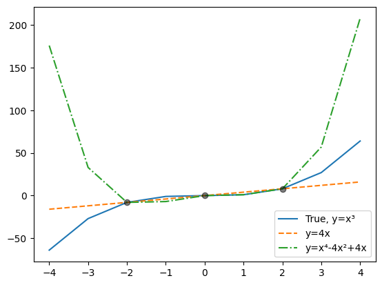
To illustrate, consider a simple data-generating process where \(Y\) is given by the deterministic function \(Y = X^3\) and \(X\) is uniformly distributed over \(\{-4,-3,\ldots,3,4\}\). Let’s take absolute error \(|y-\hat y|\) as our loss function.
Suppose we collect a small sample, say: \[
\{\,(-2,-8),\,(0,0),\,(2,8)\}.
\]
Putting ourselves in the place of a machine learning practitioner who does not know the true data generating process, and has only this sample to workd with, we try to find a good predictor of \(Y\) by minimizing empirical risk over the sample. Say, we choose as our model all 4th-degree polynomials: \[
\phi(x,\beta_0,\ldots,\beta_4) \;=\; \beta_4\,x^4 + \ldots + \beta_1\,x + \beta_0.
\]
Two functions from this class are \(y = 4x\) and \(y = x^4 - 4x^2 + 4x\). The code below plots these two functions over the full set \(\{-4,\ldots,4\}\), highlighting the sample points:
Both functions perfectly fit our sample points, giving \(\hat{R}_n(\beta)=0\) on those three points. Yet they behave very differently on the rest of the domain, so their true risks \(R(\beta)\) differ widely. From the sample alone, we would have no way of knowing which is better over the full set of \(X\) values.
Notice something even more ironic: the true function \(y=x^3\) is itself within our model family, so the approximation error for our model is zero. Yet the true function does no better on our sample than the other two polynomials. No one could fault us for picking one of them instead of the true function. But if we did that we would end up with a non-zero estimation error.
2.2.1 No Free Lunch Theorems
What can we do to avoid such traps on real data (not artificially generated examples)? Unfortunately, there exist impossibility theorems called No Free Lunch Theorems which show that for each finite-data learning algorithm, howsoever clever, there exists some distributions \(\mathcal{D}\) on which that algorithm fails. Thus, if we truly assume \(\mathcal{D}\) can be anything, we must accept the possibility of failure.
The good news is that if we have some prior information that tells us that \(\mathcal{D}\) belongs to a restricted family of distributions, we can incorporate that knowledge into our modeling and avoid failure. We could do this by picking a model or predictor class tuned to this restricted class. Or we could tune the way we use the data to pick a parameter value or predictor. This use of background knowledge to constrain our hypothesis space is sometimes called inductive bias. Far from being a bad word, this kind of “bias” is good: by narrowing our search, we can learn from a finite sample about the infinite domain.
2.3 Overfitting
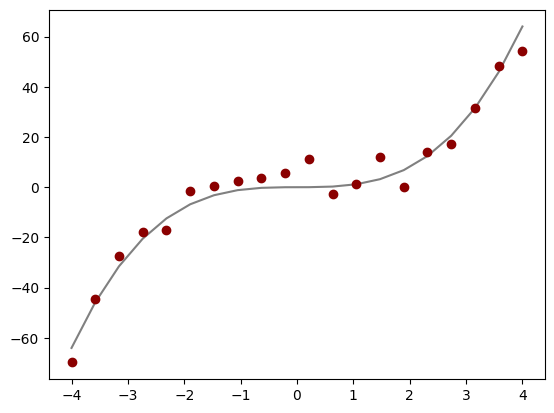
Overfitting is a specific manifestation of the learning problem, especially in the presence of noise. For instance, let \[
Y \;=\; X^3 \;+\; \epsilon,
\] where \(\epsilon\) is a noise term. The code below creates 20 sample points evenly spaced over \([-4,4]\) and adds normally distributed noise with a mean of 0 and some variance:
import numpy as npimport numpy.random as nprimport matplotlib.pyplot as pltrng = npr.default_rng(100)x = np.linspace(-4,4,20)y = x**3+ rng.normal(size=20)*5plt.plot(x, x**3, color="grey")plt.plot(x, y, "o", color="darkred")plt.show()
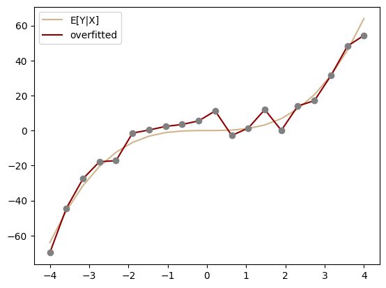
Now suppose we let a very flexible model (a 20th-degree polynomial) try to fit this noisy sample with ordinary least squares:
from sklearn.linear_model import LinearRegressionX = np.vstack([x**n for n inrange(1,21)]).Tmodel = LinearRegression()model.fit(X, y)yhat = model.predict(X)plt.plot(x, x**3, "-", color="tan", label="E[Y|X]")plt.plot(x, yhat, "-", color="darkred", label="overfitted")plt.plot(x, y, "o", color="grey")plt.legend()plt.show()
The code above uses scikit-learn’s LinearRegression class, which implements ordinary least squares regression. Like most scikit-learn model classes, it follows a consistent interface pattern: first we create a model instance with model = LinearRegression(), then call its fit() method with training data to estimate parameters, and finally use predict() to make predictions on new data. The fit() method takes a matrix of regressors X (one column per regressor, one row per observation, as you may already be familiar with from your econometrics courses) and target vector y as arguments, estimates the model parameters, and stores them internally. The predict() method takes a feature matrix and returns predicted values using those fitted parameters. This pattern of instantiate-fit-predict is standard across scikit-learn’s supervised learning models, making it easy to swap in different algorithms while keeping the same code structure. Here, we construct our feature matrix X by stacking powers of x up to degree 20, effectively fitting a high-degree polynomial.
We see that the fitted curve almost exactly passes through the training points but in order to do so it oscillates wildly between them. This is overfitting: the model has learned not just the underlying pattern but also the random noise in our training data. It thus achieves a very low \(\hat{R}_n\), but its true risk \(R\) is actually worse than \(E[Y|X] = X^3\) (tan line) curve which is the best predictor for the squared error loss. The oscillations occur because the high-degree polynomial is flexible enough to chase every small fluctuation in the sample.
2.4 The Train–Test Split: A Partial Solution
A common way to detect overfitting is to set aside a part of the original data as a test set. We use the remaining training set to estimate the model parameters, and then measure performance on the test set to get an independent estimate of \(R\). Since the test set did not play any role in fitting, it can act as an independent estimator of the true risk of an estimate and thus expose overfitting.
In scikit-learn, the function train_test_split randomly splits the data into training and test sets. The test_size=0.2 parameter reserves 20% of the data for testing, while random_state=100 ensures reproducible splits by fixing the random seed:
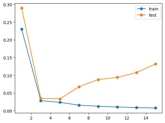
We can then fit polynomials of increasing degree to the training set and compare their performance on both training and test sets. The code below iterates through polynomial degrees from 1 to 15 (in steps of 2), fits each model to the training data, and computes the mean squared error (MSE) on both training and test sets. This allows us to visualize how model complexity affects performance on seen versus unseen data:
model_orders = np.arange(1,16,2)train_mse = np.empty_like(model_orders,dtype=float)test_mse = np.empty_like(model_orders,dtype=float)for i, n inenumerate(model_orders): X_train = np.vstack([x_train**m for m inrange(1,n+1)]).T model = LinearRegression() model.fit(X_train, y_train) yhat_train = model.predict(X_train) train_mse[i] = ((y_train - yhat_train)**2).mean() X_test = np.vstack([x_test**m for m inrange(1,n+1)]).T yhat_test = model.predict(X_test) test_mse[i] = ((y_test - yhat_test)**2).mean()plt.plot(model_orders, train_mse, "o-", label="train")plt.plot(model_orders, test_mse, "o-", label="test")plt.legend()plt.show()
The plot above shows what is known as a training curve - a visualization of how model performance changes with increasing model complexity. By plotting both training and test error, it reveals the relationship between model complexity and generalization. The training curve clearly illustrates:
Training Error: Decreases with model complexity (degree). A sufficiently flexible model can fit every nuance of the training set, potentially driving training error close to zero.
Test Error: Initially goes down as the model starts capturing genuine patterns, but then eventually goes up as it begins fitting noise. The point where test error is lowest suggests the optimal model complexity.
These curves vividly demonstrate the fundamental tradeoff in ML: we want models complex enough to capture real patterns but simple enough to avoid fitting the noise.
In practice instead of just splitting the data into training and test sets, we do a threefold split into training, validation and test sets. We use the training set to fit models. Then we use the error on the validation set to choose between models, maybe using a training curve like the above with the validation error instead of the training error. Finally we use the test data to get an estimate of the risk of the model finally chosen.
This hierarchy of use of the three sets must be strictly followed. If the estimation step can look at the validation set, it can adapt to the nuances in the validation set, thus invalidating it as a independent yardstick to be used in model choice. Similarly if the model choice step looks at the test set, it invalidated its independence.
The firewalling of the three sets from one another must be observed by the analyst too. To keep their results meaningful they must resist the temptation to check thei performance of a model on the test set before choosing a model.
Data kept aside for validation or test is not used in estimating the model. Since more data reduces the estimation error we don’t want to keep these two sets too large. On the other hand we don’t want to keep them too small either since we are using them as proxies for the distribution \(\mathcal{D}\), relying on the law of large numbers, and that provides a good approximation only for large sample sizes.
Later we will learn about the techinque of cross-validation that uses data more efficiently than this three-fold split.
2.5 The Bias–Variance Tradeoff
Sometime in machine learning discussions you may come across the term bias–variance tradeoff. This is a way of decomposing the error of a predictor in the case of the squared error loss function, and it is complementary to the approximation/estimation error decomposition we have discussed. When predicting a true function \(f(x)\) with some estimator \(\hat{f}(x)\) under squared loss, one can decompose the expected prediction error at a point \(x\) as \[
\mathbb{E}\bigl[\bigl(Y - \hat{f}(x)\bigr)^2\bigr]
= \underbrace{\mathrm{Var}\bigl(\hat{f}(x)\bigr)}_{\text{variance}}
\;+\; \underbrace{\bigl[\mathbb{E}\bigl(\hat{f}(x)\bigr) - f(x)\bigr]^2}_{\text{(squared) bias}}
\;+\; \underbrace{\sigma^2}_{\text{irreducible noise}},
\] where \(\mathrm{Var}\bigl(\hat{f}(x)\bigr)\) captures how much the learned function fluctuates around its mean when trained on different samples, and \(\bigl[\mathbb{E}\bigl(\hat{f}(x)\bigr) - f(x)\bigr]^2\) captures the systematic offset of its mean prediction from the truth. The last term, \(\sigma^2\), arises from inherent noise in the data.
This bias–variance decomposition expresses the same fundamental tension we described in terms of approximation and estimation errors: one must choose a model family rich enough to capture the signal (low bias) but not so flexible that it overfits the sample (high variance).
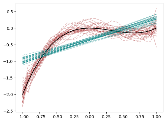
We illustrate this tradeoff concretely with an example. Suppose we take 30 different samples from \(Y = x^3 - x^2 + \text{(noise)}\). Each time, we fit an 11th-degree polynomial (brown) and a simple linear model (teal), and we plot the predicted curves:
We see the 11th-degree curves (brown) do a better job of capturing the shape of \(y = x^3 - x^2\), so they have lower bias (or smaller approximation error). In fact this function is a polynomial of degree less than 11, so it belongs to the functions among which we are looking for a empirical risk minimizer. If it happens to be chosen the only risk that remains will be from the variability contributed by the noise we have added. However the wriggly brown curves in the plot above show that it does not actually get chosen. The extra flexibility provided by the 11-th degree functional form causes the model to overfit the noise. As the noise varies from sample to sample, different 11-th degree polynomials get chosen. We get an estimation error which manifests in the form of a higher variance in the estimator from sample to sample. By contrast, the linear models (teal) cannot approximate the true curve as well (thus higher bias or larger approximation error). The best possible linear curve would still have a risk over and above that contributed by the noise because of how badly it fits the shape of the population regression curve. But it has the virtue that becuase of its rigidity it is less sensitive to the noise and thus moves around less from sample to sample (thus lower variance). The fitted lines from different samples differ little from the best possible line. They have low estimation error
This example directly illustrates how, under squared error loss, the bias–variance decomposition complements the approximation–estimation perspective. A more flexible model reduces bias (approximation error) but risks greater variance (estimation error), while a simpler model does the opposite. Balancing these two aspects remains a key theme in model building, guiding our choice of model complexity as we seek to avoid both underfitting and overfitting.
Often the bias-variance language is used in an informal way to refer to approximation vs. estimation error even when using loss functions for which strictly speaking there is no bias-variance decomposition.
2.6 Conclusion
In this chapter, we examined the fundamental conceptual issues in supervised learning: model choice, empirical risk minimization, overfitting, and the interplay between approximation error and estimation error (often described as the bias–variance tradeoff). These ideas apply to the simplest linear regression setting as well as to more complex models. They guide us as we move to richer, more flexible predictors in subsequent chapters.
A rich theoretical literature addresses the issues raised here using probability theory and other branches of mathematics. A highly recommended reference is Understanding Machine Learning by Shalev-Shwartz and Ben-David (2014), which provides a more formal and thorough introduction to these topics.
Source Code
::: {.callout-note}This is an **EARLY DRAFT**.:::# Conceptual FoundationsIn this chapter we will look at the supervised learning task in the abstract to understand the basic conceptual issues at the heart of this task. For many of our illustrations, we will use linear regression as our supervised learning technique because it is something that you are very likely already familiar with. But what we learn will have applicability to all supervised learning methods, such as decision trees and neural networks, that we shall study in later chapters.## The IngredientsEvery supervised learning problem begins with $X$ and $Y$. $Y$ is the outcome we are trying to predict; $X$ is the information we have at hand to make that prediction. When $Y$ is a *continuous* variable, we call the task **regression**; when $Y$ is a *categorical* variable, we call it **classification**. $X$ may be text, video, audio, or columns of numbers. But by the time we arrive at a mathematical model, we expect both $X$ and $Y$ to have been converted into numbers, for example by treating a video clip as an array of frames, each frame in it as an array of pixels and each pixel as a triple of red, green and blue color intensities. Similarly a paragraph of text can be converted into a series of numbers by choosing a dictionary which has a serial number for each word, and replacing each word in our paragraph by its serial number in the dictionary. A series of $d$ can in turn be thought of as a vector in a $d$-dimensional vector space. Assuming that some encoding of this sort has already been applied to our input data, we can take $\mathcal{X}$ and $\mathcal{Y}$ to be subsets of some (possibly very high dimensional) Euclidean spaces for the purposes of our subsequent analysis. Because we are learning from data, we assume we have observations of $X$ and $Y$ in the form of pairs $\bigl(x_i,y_i\bigr)$, where $i$ denotes the observation number. We typically assume that these observations are drawn independently from some common probability distribution $\mathcal{D}$. This is often abbreviated by saying that they are “independent and identically distributed (IID).” The distribution $\mathcal{D}$ is not known to us. Indeed, our entire project is to learn about the conditional distribution $P(Y\mid X)$ so that we can make good predictions of $Y$ given $X$. We also need to know something about the marginal distribution of $X$ to understand which regions of the input space to focus on more.The IID assumption will not always be true. For example if our observations are a time-series of observations from some real world dynamical process, say the level of water each month in a dam reservoir, then the observations close in time are likely to be correlated with each other. Or, to take another example, if it is data about the incidence of some infectious disease in households then we are likely to see correlation among neighbouring households dues to ease of disease transmission.While machine learning has been very successfully applied to time-series and other correlated data, the theoretical analysis of non-IID data generating processes in harder than that of IID processes and we shall not touch upon it in this text.In our analysis we shall assume that the new $(X,Y)$ for which our model will have to make prediction after the training phase will come from the same distribution as the distribution $\mathcal{D}$ which generated our training data. Relaxing this assumption is an active area of machine learning reasearch. This is of special interest to economists, since economists are often interested in the effects of changing the world by modifying policies. That is, they are interested in **counterfactuals**. Now, data gathered from one world cannot provide any guidance to a completely different world. So the counterfactual problem cannot be solved in full generality. But the hope is that if we restrict ourselves to particular changes, and if we have information beyond the data about how the world is put together, we may be able to make predictions for some counterfactual experiments. We will come back to this problem of counterfactual prediction in later parts of this book. For now we will restrict ourselves to the classical machine learning setting in which predictions have to be made in the same environment in which learning happened.### Parametric modelsThe task of supervised learning is to use the data to select a predictor $f\colon \mathcal{X} \to \mathcal{Y}$ from some class of predictors $\mathcal{F}$ that captures the patterns in the distribution $\mathcal{D}$ well.For many machine learning methods used in practice, the class of potential predictors $\mathcal{F}$ takes the structured form of a **parametric model**. This is a *single* function of the form $y = \phi(x;\beta)$ where $\phi \colon \mathcal{X}\times \mathcal{B} \to \mathcal{Y}$, where $\mathcal{B}$ is the space of **parameter** values. Every choice of $\beta \in \mathcal{B}$ gives us a potentially different predictor $f(x) = \phi(x,\beta)$ which can be used to predict a value $y$ for a given value of $x$. Our task now becomes one of using the data we have to find a value of $\beta$ that makes $f(x) = \phi(x,\beta)$ a good predictor.For example, if $x$ consists of observations on $k$ variables $\bigl(x^{(1)},\ldots,x^{(k)}\bigr)$, we may choose the linear regression model$$\beta_1\,x^{(1)} \;+\;\dots\;+\;\beta_k\,x^{(k)}$$and try to find a ‘good’ value for the $\beta$s.### Loss Functions and RiskTo proceed, we need a way of judging how good a prediction is. In an ideal world, we would predict a value of $y$ that matches the true value exactly. But this is generally not possible:1. $Y$ may depend on variables beyond $X$. 2. $Y$ may be affected by genuinely random noise. 3. Even if $Y$ were a deterministic function of $X$, we might be unable to figure out the exact function and thus may have to choose among imperfect solutions.Hence we introduce a **loss function** $L(y,\hat{y})$ that captures the cost of predicting $\hat{y}$ when the true value is $y$. In principle, $L$ should reflect the real-world cost of a bad prediction. In practice, such principled cost functions are often unavailable, so we resort to more conventional loss functions like the squared loss $\bigl(y-\hat{y}\bigr)^2$ or absolute loss $\bigl|y - \hat{y}\bigr|$ for regression.Given a loss function, we define the **expected risk** or **generalization error** of a predictor $f$ as$$R(f) \;=\; \mathbb{E}_{\mathcal{D}}\bigl[L\bigl(Y,\,f(X)\bigr)\bigr].$$This expectation is with respect to the unknown data-generating distribution $\mathcal{D}$. In the parametric context, the risk of a parameter value $\beta$ is$$R(\beta) \;=\; \mathbb{E}_{\mathcal{D}}\!\bigl[L\bigl(Y,\,\phi\bigl(X,\beta\bigr)\bigr)\bigr].$$The optimal predictor $f^*$, or the optimal $\beta^*$, would minimize this expected risk.### Empirical Risk MinimizationHowever, $\mathcal{D}$ is unknown, so we cannot directly compute $R(\beta)$. We only have the sample $\bigl(x_i,y_i\bigr)$. A natural idea is therefore to minimize the **empirical risk**, that is, the sample average of the loss:$$\hat{R}_n(\beta) \;=\; \frac{1}{n}\sum_{i=1}^n L\!\bigl(y_i,\,\phi\bigl(x_i,\beta\bigr)\bigr).$$**Empirical risk minimization (ERM)** is a general machine learning approach that, given a class of candidate predictors or a parametric model, tries to choose a predictor that minimizes the empirical risk. Because our data are IID, the hope is that by minimizing $\hat{R}_n$ may come close minimizing $R$. In a regression context with squared loss, ERM is precisely ordinary least squares.ERM is not the only approach to choosing predictors, though it is a very important one.Our learning task now naturally breaks into steps:1. **Model Choice:** Choose a class of predictors $\mathcal{F}$ or a parametric model $\phi$. The minimum risk $R(f)$ or $R(\beta)$ achievable by a predictor in this class of model is called its **approximation error**. It captures how well this model can approximate the pattern in $\mathcal{D}$ in the best-case scenario. Since we don't have complete knowledge of $\mathcal{D}$ this error is not directly observable. However, conceptually we can see that the greater the variety of predictors available in our class or model, the less the approximation error is likely to be. Why not choose our class to be *all* functions from $\mathcal{X}$ to $\mathcal{Y}$ and thereby guarantee ourselves the least possible approximation error? We will see in a minute why this may not be a good idea.2. **Estimation:** Since we have access not to $\mathcal{D}$ but only to a finite sample from it, we cannot directly choose the best predictor from a given model. Instead we use some indirect method such as empirical risk minimization to find a predictor which we hope will be good. This is the estimation or training step in machine learning. Since our methods work only with a finite sample, the predictor we choose is likely to be inferior to the best possible predictor. The gap between the risk of our chosen predictor and the best predictor in the model is the **estimation error**.If $\beta^*$ is the (unknown) value that minimizes risk for a given model, and $\beta$ is parameter value we choose, then we have$$R(\beta)= \underbrace{R(\beta^*)}_{\text{approximation error}}\;+\;\underbrace{R(\beta) - R(\beta^*)}_{\text{estimation error}},$$## The Problem of LearningLet us come back to the question of why we don't choose the most flexible possible predictor class $\mathcal{F}$, the class of all functions from $\mathcal{X} \to \mathcal{Y}$? This would guarantee us the least possible approximation error.One reason we don't do so is practical. The class of all functions from $\mathcal{X}$ to $\mathcal{Y}$ can be enormous. We may have no efficient methods to even approximately minimize empirical risk over this entire class. We would like to work withing a restricted class of function where finding (at least approximately) the empirical risk minimizer can be accomplished in a usefully short amount of time.However, there is a deeper conceptual reason why we cannot make our class of candidate predictors too large our our parametric model too flexible.A little reflection shows that approximation error and estimation error are not independent; there is likely to be a **tradeoff** between them. By making our model $\phi$ more flexible and complex, we reduce approximation error, since it becomes more likely that one of the functions in that richer family can capture the pattern in $\mathcal{D}$ well. But higher complexity can worsen estimation error because our finite sample becomes worse at guiding us about the behaviour of predictors over the whole domain. A predictor which is inferior in the sample can turn out to be far superior over the entire domain since now. In other words the estimation error may blow up.To illustrate, consider a simple data-generating process where $Y$ is given by the deterministic function $Y = X^3$ and $X$ is uniformly distributed over $\{-4,-3,\ldots,3,4\}$. Let's take absolute error $|y-\hat y|$ as our loss function.Suppose we collect a small sample, say:$$\{\,(-2,-8),\,(0,0),\,(2,8)\}.$$Putting ourselves in the place of a machine learning practitioner who does not know the true data generating process, and has only this sample to workd with, we try to find a good predictor of $Y$ by minimizing empirical risk over the sample. Say, we choose as our model all 4th-degree polynomials:$$\phi(x,\beta_0,\ldots,\beta_4) \;=\; \beta_4\,x^4 + \ldots + \beta_1\,x + \beta_0.$$Two functions from this class are $y = 4x$ and $y = x^4 - 4x^2 + 4x$. The code below plots these two functions over the full set $\{-4,\ldots,4\}$, highlighting the sample points:```{python}#| eval: trueimport numpy as npimport matplotlib.pyplot as pltx = np.arange(-4,5,1)y = x**3x_train = x[[2,4,6]] # [-2, 0, 2]y_train = y[[2,4,6]] # [-8, 0, 8]plt.plot(x, y, "-", label="True, y=x³")plt.plot(x, 4*x, "--", label="y=4x")plt.plot(x, x**4-4*x**2+4*x, "-.", label="y=x⁴-4x²+4x")plt.plot(x_train, y_train, "o", color="black", alpha=0.5)plt.legend()plt.show()```Both functions perfectly fit our sample points, giving $\hat{R}_n(\beta)=0$ on those three points. Yet they behave very differently on the rest of the domain, so their true risks $R(\beta)$ differ widely. From the sample alone, we would have no way of knowing which is better over the full set of $X$ values.Notice something even more ironic: the true function $y=x^3$ is itself within our model family, so the approximation error for our model is zero. Yet the true function does no better on our sample than the other two polynomials. No one could fault us for picking one of them instead of the true function. But if we did that we would end up with a non-zero estimation error.### No Free Lunch TheoremsWhat can we do to avoid such traps on real data (not artificially generated examples)? Unfortunately, there exist impossibility theorems called **No Free Lunch Theorems** which show that for each finite-data learning algorithm, howsoever clever, there exists some distributions $\mathcal{D}$ on which that algorithm fails. Thus, if we truly assume $\mathcal{D}$ can be anything, we must accept the possibility of failure.The good news is that if we have *some prior information* that tells us that $\mathcal{D}$ belongs to a restricted family of distributions, we can incorporate that knowledge into our modeling and avoid failure. We could do this by picking a model or predictor class tuned to this restricted class. Or we could tune the way we use the data to pick a parameter value or predictor. This use of background knowledge to constrain our hypothesis space is sometimes called **inductive bias**. Far from being a bad word, this kind of “bias” is *good*: by narrowing our search, we can learn from a finite sample about the infinite domain.## OverfittingOverfitting is a specific manifestation of the learning problem, especially in the presence of noise. For instance, let$$Y \;=\; X^3 \;+\; \epsilon,$$where $\epsilon$ is a noise term. The code below creates 20 sample points evenly spaced over $[-4,4]$ and adds normally distributed noise with a mean of 0 and some variance:```{python}#| eval: trueimport numpy as npimport numpy.random as nprimport matplotlib.pyplot as pltrng = npr.default_rng(100)x = np.linspace(-4,4,20)y = x**3+ rng.normal(size=20)*5plt.plot(x, x**3, color="grey")plt.plot(x, y, "o", color="darkred")plt.show()```Now suppose we let a very flexible model (a 20th-degree polynomial) try to fit this noisy sample with ordinary least squares:```{python}#| eval: truefrom sklearn.linear_model import LinearRegressionX = np.vstack([x**n for n inrange(1,21)]).Tmodel = LinearRegression()model.fit(X, y)yhat = model.predict(X)plt.plot(x, x**3, "-", color="tan", label="E[Y|X]")plt.plot(x, yhat, "-", color="darkred", label="overfitted")plt.plot(x, y, "o", color="grey")plt.legend()plt.show()```The code above uses scikit-learn's `LinearRegression` class, which implements ordinary least squares regression. Like most scikit-learn model classes, it follows a consistent interface pattern: first we create a model instance with `model = LinearRegression()`, then call its `fit()` method with training data to estimate parameters, and finally use `predict()` to make predictions on new data. The `fit()` method takes a matrix of regressors `X` (one column per regressor, one row per observation, as you may already be familiar with from your econometrics courses) and target vector `y` as arguments, estimates the model parameters, and stores them internally. The `predict()` method takes a feature matrix and returns predicted values using those fitted parameters. This pattern of instantiate-fit-predict is standard across scikit-learn's supervised learning models, making it easy to swap in different algorithms while keeping the same code structure. Here, we construct our feature matrix `X` by stacking powers of `x` up to degree 20, effectively fitting a high-degree polynomial. We see that the fitted curve almost exactly passes through the training points but in order to do so it oscillates wildly between them. This is **overfitting**: the model has learned not just the underlying pattern but also the random noise in our training data. It thus achieves a very low $\hat{R}_n$, but its true risk $R$ is actually worse than $E[Y|X] = X^3$ (tan line) curve which is the best predictor for the squared error loss. The oscillations occur because the high-degree polynomial is flexible enough to chase every small fluctuation in the sample.## The Train–Test Split: A Partial SolutionA common way to detect overfitting is to set aside a part of the original data as a **test set**. We use the remaining **training set** to estimate the model parameters, and then measure performance on the test set to get an independent estimate of $R$. Since the test set did not play any role in fitting, it can act as an independent estimator of the true risk of an estimate and thus expose overfitting.In `scikit-learn`, the function `train_test_split` randomly splits the data into training and test sets. The `test_size=0.2` parameter reserves 20% of the data for testing, while `random_state=100` ensures reproducible splits by fixing the random seed:```{python}#| eval: truefrom sklearn.model_selection import train_test_splitx2 = np.linspace(-1,1,25)y2_true = x2**3- x2**2rng = npr.default_rng(100)y2 = y2_true + rng.normal(size=25)*0.2x_train, x_test, y_train, y_test = train_test_split( x2, y2, test_size=0.2, random_state=100)```We can then fit polynomials of increasing degree to the training set and compare their performance on both training and test sets. The code below iterates through polynomial degrees from 1 to 15 (in steps of 2), fits each model to the training data, and computes the mean squared error (MSE) on both training and test sets. This allows us to visualize how model complexity affects performance on seen versus unseen data:```{python}#| eval: truemodel_orders = np.arange(1,16,2)train_mse = np.empty_like(model_orders,dtype=float)test_mse = np.empty_like(model_orders,dtype=float)for i, n inenumerate(model_orders): X_train = np.vstack([x_train**m for m inrange(1,n+1)]).T model = LinearRegression() model.fit(X_train, y_train) yhat_train = model.predict(X_train) train_mse[i] = ((y_train - yhat_train)**2).mean() X_test = np.vstack([x_test**m for m inrange(1,n+1)]).T yhat_test = model.predict(X_test) test_mse[i] = ((y_test - yhat_test)**2).mean()plt.plot(model_orders, train_mse, "o-", label="train")plt.plot(model_orders, test_mse, "o-", label="test")plt.legend()plt.show()```The plot above shows what is known as a **training curve** - a visualization of how model performance changes with increasing model complexity. By plotting both training and test error, it reveals the relationship between model complexity and generalization. The training curve clearly illustrates:1. **Training Error:** Decreases with model complexity (degree). A sufficiently flexible model can fit every nuance of the training set, potentially driving training error close to zero. 2. **Test Error:** Initially goes down as the model starts capturing genuine patterns, but then eventually goes *up* as it begins fitting noise. The point where test error is lowest suggests the optimal model complexity.These curves vividly demonstrate the fundamental tradeoff in ML: we want models complex enough to capture real patterns but simple enough to avoid fitting the noise.In practice instead of just splitting the data into training and test sets, we do a threefold split into **training**, **validation** and **test** sets. We use the training set to fit models. Then we use the error on the validation set to choose between models, maybe using a training curve like the above with the validation error instead of the training error. Finally we use the test data to get an estimate of the risk of the model finally chosen.This hierarchy of use of the three sets must be strictly followed. If the estimation step can look at the validation set, it can adapt to the nuances in the validation set, thus invalidating it as a independent yardstick to be used in model choice. Similarly if the model choice step looks at the test set, it invalidated its independence.The firewalling of the three sets from one another must be observed by the analyst too. To keep their results meaningful they must resist the temptation to check thei performance of a model on the test set before choosing a model.Data kept aside for validation or test is not used in estimating the model. Since more data reduces the estimation error we don't want to keep these two sets too large. On the other hand we don't want to keep them too small either since we are using them as proxies for the distribution $\mathcal{D}$, relying on the law of large numbers, and that provides a good approximation only for large sample sizes.Later we will learn about the techinque of cross-validation that uses data more efficiently than this three-fold split.## The Bias–Variance TradeoffSometime in machine learning discussions you may come across the term **bias–variance tradeoff**. This is a way of decomposing the error of a predictor in the case of the squared error loss function, and it is complementary to the approximation/estimation error decomposition we have discussed. When predicting a true function $f(x)$ with some estimator $\hat{f}(x)$ under squared loss, one can decompose the expected prediction error at a point $x$ as$$\mathbb{E}\bigl[\bigl(Y - \hat{f}(x)\bigr)^2\bigr]= \underbrace{\mathrm{Var}\bigl(\hat{f}(x)\bigr)}_{\text{variance}} \;+\; \underbrace{\bigl[\mathbb{E}\bigl(\hat{f}(x)\bigr) - f(x)\bigr]^2}_{\text{(squared) bias}} \;+\; \underbrace{\sigma^2}_{\text{irreducible noise}},$$where $\mathrm{Var}\bigl(\hat{f}(x)\bigr)$ captures how much the learned function fluctuates around its mean when trained on different samples, and $\bigl[\mathbb{E}\bigl(\hat{f}(x)\bigr) - f(x)\bigr]^2$ captures the systematic offset of its mean prediction from the truth. The last term, $\sigma^2$, arises from inherent noise in the data.This **bias–variance decomposition** expresses the same fundamental tension we described in terms of approximation and estimation errors: one must choose a model family rich enough to capture the signal (low bias) but not so flexible that it overfits the sample (high variance). We illustrate this tradeoff concretely with an example. Suppose we take 30 different samples from $Y = x^3 - x^2 + \text{(noise)}$. Each time, we fit an 11th-degree polynomial (brown) and a simple linear model (teal), and we plot the predicted curves:```{python}#| eval: truex3 = np.linspace(-1,1,25)y3_true = x3**3- x3**2import numpy as npimport numpy.random as nprrng = npr.default_rng(100)X3 = np.vstack([x3**d for d inrange(1,11)]).Tfor _ inrange(30): y3 = y3_true + rng.normal(size=25)*0.2from sklearn.linear_model import LinearRegression model = LinearRegression() model.fit(X3, y3) yhat3 = model.predict(X3) plt.plot(x3, yhat3, "--", color='brown', alpha=0.3)plt.plot(x3, y3_true, "-", color="black")X3lin = x3[:, np.newaxis]for _ inrange(30): y3 = y3_true + rng.normal(size=25)*0.2 model = LinearRegression() model.fit(X3lin, y3) yhat3 = model.predict(X3lin) plt.plot(x3, yhat3, "--", color='teal', alpha=0.3)```We see the 11th-degree curves (brown) do a better job of capturing the *shape* of $y = x^3 - x^2$, so they have **lower bias** (or **smaller approximation error**). In fact this function is a polynomial of degree less than 11, so it belongs to the functions among which we are looking for a empirical risk minimizer. If it happens to be chosen the only risk that remains will be from the variability contributed by the noise we have added. However the wriggly brown curves in the plot above show that it does not actually get chosen. The extra flexibility provided by the 11-th degree functional form causes the model to overfit the noise. As the noise varies from sample to sample, different 11-th degree polynomials get chosen. We get an estimation error which manifests in the form of a **higher variance** in the estimator from sample to sample. By contrast, the linear models (teal) cannot approximate the true curve as well (thus **higher bias** or **larger approximation error**). The best possible linear curve would still have a risk over and above that contributed by the noise because of how badly it fits the shape of the population regression curve. But it has the virtue that becuase of its rigidity it is less sensitive to the noise and thus moves around less from sample to sample (thus **lower variance**). The fitted lines from different samples differ little from the best possible line. They have low **estimation error**This example directly illustrates how, under squared error loss, the bias–variance decomposition complements the approximation–estimation perspective. A more flexible model reduces bias (approximation error) but risks greater variance (estimation error), while a simpler model does the opposite. Balancing these two aspects remains a key theme in model building, guiding our choice of model complexity as we seek to avoid both underfitting and overfitting.Often the bias-variance language is used in an informal way to refer to approximation vs. estimation error even when using loss functions for which strictly speaking there is no bias-variance decomposition.## ConclusionIn this chapter, we examined the fundamental conceptual issues in supervised learning: model choice, empirical risk minimization, overfitting, and the interplay between approximation error and estimation error (often described as the bias–variance tradeoff). These ideas apply to the simplest linear regression setting as well as to more complex models. They guide us as we move to richer, more flexible predictors in subsequent chapters.A rich theoretical literature addresses the issues raised here using probability theory and other branches of mathematics. A highly recommended reference is *[Understanding Machine Learning](https://www.cs.huji.ac.il/~shais/UnderstandingMachineLearning/)* by Shalev-Shwartz and Ben-David (2014), which provides a more formal and thorough introduction to these topics.---