Neural networks have emerged as one of the most powerful and versatile tools in modern machine learning. While they had been studied since the mid-20th century, it is only in the 21st that they have truly come into their own. Among machine learning models they have been able to get the most performance improvement out of advances in hardware and algorithms and the availability of massive data sets. Today, neural networks achieve state-of-the-art performance across diverse domains from computer vision to natural language processing. Most significantly, neural networks are at the core of the large language models which have radically changed the AI landscape in the last few years. It can be argued that knowing something about them is as essential for an educated person now as knowing something about atoms or cells.
Apart from the remarkable practical utility, neural networks have two remarkable features that make them fascinating subjects of study. First, they are built up from very simple constituent parts, the so-called units. Each unit compute a simple mathematical operations that would be understandable to a high-schooler. The entire complexity and power of neural network models comes from connecting a very large number of these units together. Thus the predictive power of neural networks is an example of an emergent phenomena, where collectives exhibit properties which are not simply the sum of the properties of individual parts.
The second remarkable property of neural networks is that stochastic gradient descent (SGD) and its variants are successful in training very complex networks with billions of parameters. As you would remember from the optimization chapter, SGD is a stepwise minimization algorithm that move in the direction opposite to the gradient in each step. We expect it to succeed on convex (i.e. bowl shaped) functions where if you take steps in the ‘downward’ direction slowly enough, you’ll ultimate reach the global minimum. The functions represented by neural network are, however, not convex. And yet SGD seems to do very well in minimizing them.
There is more. While SGD works well, it somehow also manages not to work too well for its own good when it comes to overfitting. If you recall our discussion in the regression chapter, when we added many higher-order polynomial regressors, our model overfit the noise in the data and has worse test performance than simpler models. Neural networks on the other hand are much more robust to overparametrization. Even if a neural network has enough flexibility to overfit training data, when trained with SGD it somehow manages not to do so and retains good performance over test data.
Satisfactory theoretical understanding of these and other strange behaviours of neural networks trained with SGD is still to be reached. And yet their successes cannot be ignored. At the moment, therefore, we are compelled to study these phenomena empirically, through trial and error. To become a successful practitioner of machine learning using neural networks it is imperative that you begin experimenting with these models and building up an intuitive feel for their behaviour.
But before you can do that, there is some basic jargon and intuition that needs to be picked up. This chapter is dedicated to that task.
7.1 What Is a Neural Network?
A neural network is a particular kind of parametric model. As you will recall, a general parametric model is a function of the form \(y = \phi(x;\beta)\) where
\(x\) are the inputs to the model,
\(y\) are its outputs and
\(\beta\) are parameters to be learnt from the data
In fitting or training any parametric model we use data to pick values of \(\beta\) in a way that, we hope, will give us a good predictor of \(y\). Neural networks follow the same basic plan. What sets them apart is that in their case the function \(\phi\) is formed by connecting together (composing) many simple functions of a particular form called units. Each neural network unit is a function of the form:
\[ z = u(v;W,b) = \sigma(Wv+b) \]
where,
\(v\) is the input of the unit,
\(z\) its output,
\(W\) is a matrix of parameters called the weights of the unit,
\(b\) is a vector of parameters called its biases (not to be confused with bias in statistical estimation, inductive bias in learning theory, or any other kind of bias for that matter).
\(\sigma\) is a potentially nonlinear function called the activation function (again a name into which you should not read anything. It is a holdover from the past).
The weights and biases of all the units of a neural network taken together constitute the parameter set of the network.
Here is a simple neural network which takes two inputs \(x_1\) and \(x_2\) and produces a single output \(y\). \[
\begin{align*}
\text{Unit 1:}\qquad z_1 &= W_1 \begin{bmatrix}x_1\\x_2\end{bmatrix} + b_1\\
\text{Unit 2:}\qquad z_2 &= W_2 \begin{bmatrix}x_1\\x_2\end{bmatrix} + b_2\\
\text{Unit 3:}\qquad z_3 &= W_3 \begin{bmatrix}x_1\\x_2\end{bmatrix} + b_3\\
\text{Unit 4:}\qquad y &= W_4 \begin{bmatrix}z_1\\z_2\\z_3\end{bmatrix} + b_4\\
\end{align*}
\]
Here \(W_1\), \(W_2\) and \(W_3\) are matrices of dimension \(1\times 2\) and \(W_4\) is a matrix of dimension \(1 \times 3\). \(b_1\), And \(b_2\), \(b_3\) and \(b_4\) are 1-dimensional vectors, i.e. constants. The 14 numbers which make up the elements of these matrices and vectors together are the parameters of this model. We have taken the activation function to be the identity function for simplicity.
As you can see that a neural network is just functions applied to the outputs of other functions. We talk about these input output relationships in a diagrammatic language. So for this model we will say that all the inputs of the model are connected to each of the Units 1, 2 and 3. Their outputs are connected to Unit 4, whose output is the output of th model.
Here’s a diagram of the simple neural network described above:
    Inputs                Hidden Layer              Output

    x₁ ────┬─────► Unit 1 (z₁) ─┐
           │                    │
           ├─────► Unit 2 (z₂) ─┼─────► Unit 4 (y)
           │                    │
    x₂ ────┴─────► Unit 3 (z₃) ─┘
The choice of what units to include in the model and how to connect them together is called the architecture of a neural network. The architecture of a model must be chosen before its parameters can be estimated using SGD. We use common practice and experience to choose a few candidate architectures and then select between then based on their performance on actual data (validation sets, not the training sets).
In this chapter we consider only a subset of architectures known as feedforward neural networks. In these networks the units can be grouped into a sequence of layers in a way that the inputs of any unit in layer \(i\) must be be the output of a layer \(j<i\). So data in a feedforward network flows unidirectionally from inputs to outputs without any feedback.
Our example above is a feedforward network with two layers. Units 1, 2 and 3 constitute the first layer and Unit 4 the second.
The number of layers in a network is called its depth. The number of a units in a layer is its width. Layers whose outputs are only fed into other layers and do not directly constitute part of the neural network’s final output are known as hidden layers, like the first layer in our example above.
Networks with high depth (there is no set standard) are called deep networks, and machine learning using them is called deep learning.
Neural networks were originally motivated by neurobiology and some literature refers to units as neurons. But the analogies with nervous systems have not been of much use in our understanding of these models and we will not bother with them.
7.2 Units
A neural network can include units of various type. All types of units first apply a linear transformation \(Wv+b\) to the inputs (mathematicians will call them affine transformations because of the \(b\)) and then apply an activation function \(\sigma\). Different units are characterised by the \(\sigma\) function they implement. Some of the most important ones are:
7.2.1 Linear
\[\sigma(x) = x\]
Here \(\sigma\) is an identity map. In this case the unit does not apply any non-linear transformation at all. These are useful as final output units for regression models, combining the multiple outputs of the earlier layer into a single number.
7.2.2 Sigmoid
\[\sigma(z) = \frac{1}{1 + e^{-z}}\]
The non-linear transformation in a sigmoid unit maps the number \(Wv+b\) in a monotonically increasing manner into the interval \((0,1)\) It is useful as the final output unit for a model which must predict a single probability, such a binary classification models.
7.2.3 Softmax
\[
\sigma(z)_j = \frac{e^{z_j}}{\sum_{k=1}^K e^{z_k}},\quad j=1,\dots, K
\]
The softmax takes a \(K\)-dimensional input \(Wv+b\) and maps them into \(K\) non-negative numbers which add up to \(1\), with each component of the output being a monotonically increasing function of the corresponding component of the input. The softmax unit is useful as an output unit for a network which must predict \(K\) probabilities, such as a network for a multiclass classification.
The name ‘softmax’ comes from seeing this transformation as a softening of the ‘argmax’ function, where the argmax function gives an output \(1\) for the maximum component of its input and \(0\) for the other components.
7.2.4 ReLU
ReLU stands for ‘Rectified Linear Unit’. Its activation function is given by
\[
\sigma(z) = \max{0,z}
\]
The ReLU unit outputs \(0\) for negative inputs and the input itself for positive inputs. In current neural network practice ReLU units are the most common choice for hidden-layer units.
The name most probably comes from electronics, where a rectifier is a circuit which converts AC to DC. The simplest electronic rectifier just chops of the negative part of the AC waveform, just as the ReLU units chops off the negative part of its input.
For a neural network to be something more than a linear model, it must have units other than linear units. Historically, many kinds of non-linear transformations have been used in neural networks. However, at the time of writing, neural networks overwhelmingly use ReLU units in their hidden layers. Because of their simplicity ReLU units are easy to train and calculate with. And yet,remarkably, this simple type of non-linearity, employed in a multiple layers, has been found to be sufficient to model all kinds of complex patterns. Nature has been kind to us.
7.3 Universal Approximation
In a supervised learning task, we are trying to predict \(y\) given \(x\). Suppose the optimal predictor, for a given data distribution and loss function, is \(f^*(x)\). Then a basic question to ask about a model is how closely can the model approximate \(f^*\)? If a model cannot approximate \(f^*\) well at all then even with the best possible data and learning algorithm we will still suffer a loss due to the poorness of approximation. However, remember that the converse is not true. Even if the model can approximate \(f^*\) well, we may be unable to learn the parameter values that bring about this approximation and it may remain outside our reach. But let’s leave that problem for later. For the time being, let’s ask the first question. Which functions can neural networks approximate well?
Turns out the answer is any function. Neural networks are universal approximators. For any function \(f\) we can find a neural network that approximates that function arbitrarily well. In the notes to this chapter we provides notes and references to exact statements to that effect. Here we will illustrate one proof approach intuitively. Our illustration will use networks of ReLU units, since that is the most commonly used unit type currently. However universal approximation theorems can be proved for other activations such as sigmoid.
Throughout this discussion we will define \(\text{relu}(x) = \max(x,0)\).
Our goal is to approximate an arbitrary function to an arbitrary degree of accuracy. We’ll begin with simple building block and slowly build up the complexity.
7.3.1 Approximating a step function
We will begin by trying to approximate the step function:
This is a discontinuous function, and since ReLU and affine transformations are both continuous functions, no ReLU network can exactly match it. But we can approximate it arbitrarily well by subtracting one ReLU from another. Think for a minute how you might do so before you work through the example below.
Here’s one way to do it. For any \(M>0\) define the function:
Let’s look at the value of this function in different intervals:
Interval
\(\text{relu}(-Mx-1)\)
\(\text{relu}(-Mx)\)
\(\text{ramp}_M(x)\)
\(x\le -1/M\)
\(-Mx-1\)
\(-Mx\)
\(0\)
\(-1/M\le x \le 0\)
\(0\)
\(-Mx\)
\(Mx+1\)
\(0 \le x\)
\(0\)
\(0\)
\(1\)
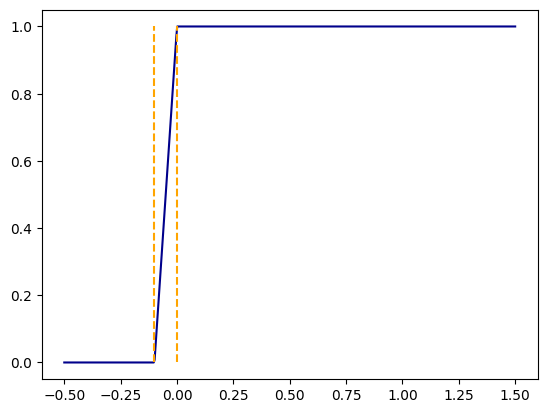
So the function takes the value \(0\) for \(x\le -1/M\) and \(1\) for \(x \ge 0\) with a linear ramp connecting the two segments. By making \(M\) larger we can make the ramp as steep as we want and get as good an approximation of the step function as we like. The code below plots this function for \(M=10\).
import numpy as npimport matplotlib.pyplot as pltx = np.linspace(-0.5,1.5,500)M =10def relu(x):return np.maximum(0,x)def ramp(x,M):return relu(-M*x-1)-relu(-M*x)+1y = ramp(x,M)plt.plot(x,y,color="darkblue")plt.vlines([-1/M,0],0,1,color="orange",linestyles="--")
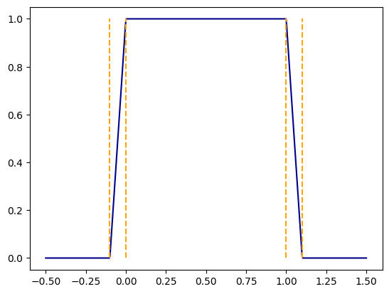
Once again because of the discontinuity we cannot exactly match this function by a composition of affine and ReLU transformations. But we can approximate it arbitrarily well by taking the ramp function we constructed above and subtracting from it a ramp shifted to the right. We define
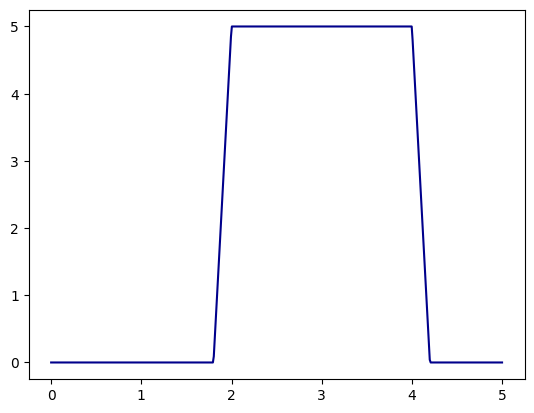
Also note that once we have an indicator function for the unit interval, we can produce a function that takes any constant value over any interval by applying affine transformations to the inputs and outputs of the unit indicator functions. To illustrate the example below plots a functions that take on the value \(5\) in the interval \([2,4]\). Figure out why it works.
x = np.linspace(0,5,500)y = unit_indicator((x-2)/2,M)*5plt.plot(x,y,color="darkblue")
7.3.3 Arbitrary functions
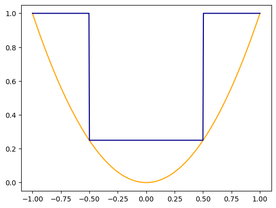
Now if we are required to approximate an arbitrary function, we break it its domain into intervals and approximate it by an indicator-like function in each interval. We illustrate by approximating the function \(f(x)=x^2\) in the domain \([-1,1]\) by approximating it by \(1\) in \([-1,-1/2]\), \(1/4\) in \([-1/2,1/2]\) and \(1\) again in \([1/2,1]\). We take \(M=1000\) to make our approximation better.
x = np.linspace(-1,1,500)true_y = x**2plt.plot(x,true_y,color="orange")approx_y = (unit_indicator((x+1)*2,1000)+(1/4)*unit_indicator((x+1/2),1000)+unit_indicator((x-1/2)*2,1000))plt.plot(x,approx_y,color="darkblue")
By splitting the domain into a larger number of smaller intervals, we can make the approximation as accurate as we wish.
The idea of these demonstrations can be extended to higher dimensions by building up higher-dimensional analogues of ramps and approximate indicator functions. The details can be found in the references.
7.3.4 Caveats
We hope to have convinced you that any (well-behaved) function can be approximated arbitrarily well by some neural network. But it is essential to put this result in the correct perspective. In the machine learning context, we are trying to approximate an unknown function. So we have no idea a priori of the architecture that would provide a good approximation to the data. In fact we don’t even have any idea of just how many neurons may be needed to get a given accuracy of approximation. Neither is there any guarantee that even if we were to somehow hit upon the right architecture we will be able to learn a good set of parameters from the data. Therefore, there is a long distance to go from showing universal approximation to having guarantees of successful learning. But it is a reassuring first step.
7.4 The Miracle/Puzzle of Deep learning
The great successes of neural networks in recent times have come from the adoption of deep architectures, i.e. architectures with many layers. While we do not have a complete understanding of why deep architectures perform so much better than shallower ones, empirical research has revealed several key advantages that help explain their remarkable performance.
7.4.1 Hierarchical feature learning
Deep networks excel at learning hierarchical representations - where each layer builds increasingly complex features by combining simpler patterns from previous layers. This mirrors how many real-world phenomena are organized: simple elements combine to form intermediate concepts, which in turn combine to form more abstract concepts.
For example, in image recognition:
Early layers detect edges and simple textures
Middle layers combine these to recognize shapes and parts
Later layers identify complete objects and their relationships
Similarly, when predicting income from worker characteristics:
Early layers might detect basic patterns like “education > 16 years” or “experience > 10 years”
Middle layers could combine these to identify “skilled professional” or “management track”
Deeper layers might recognize complex socioeconomic patterns like “high-growth career trajectory” or “industry leadership potential”
This hierarchical structure allows deep networks to efficiently represent complex functions with fewer parameters than would be required by shallow networks. A shallow network would need exponentially more neurons to capture the same relationships.
7.4.2 Inductive biases of depth
Deep architectures encode certain “inductive biases” - assumptions about what kinds of functions are likely to occur in the real world. Research has shown that deep networks naturally favor learning functions that exhibit:
Compositional structure - where complex patterns are built from simpler ones
Smoothness with local variation - functions that are generally smooth but can have sharp transitions in specific regions
Invariance to certain transformations - like recognizing objects regardless of position or lighting
These biases align well with the structure of many real-world problems, from image recognition to natural language processing to economic forecasting.
7.4.3 Optimization advantages
Counterintuitively, despite having more parameters and a more complex loss landscape, deep networks are often easier to optimize than shallow ones. Recent theoretical work suggests several ways in which this works:
Shortcut learning - Deep networks can find efficient “shortcuts” through parameter space during training. Research has shown that during optimization, networks often first learn simple patterns that explain a large portion of the data before refining their understanding with more complex patterns. This progressive learning behavior means that even though the theoretical search space is enormous, the optimization process follows a much more direct path than random exploration would suggest. For example, when training on image data, networks typically learn to detect edges and basic shapes in early training before moving on to more complex object parts. This natural curriculum helps the network avoid getting stuck in poor local minima.
Implicit regularization - SGD naturally biases solutions toward simpler functions even without explicit regularization. Research has demonstrated that the noise in mini-batch gradients, combined with a proper learning rate schedule, helps SGD avoid overly complex solutions that would fit the training data perfectly but generalize poorly. This is similar to how a hiker might avoid small, jagged paths (complex solutions) in favor of smoother trails (simpler solutions) when navigating through foggy conditions (noisy gradients).
Loss landscape geometry - The loss landscape of deep networks, while non-convex, often contains many good local minima that are nearly equivalent in performance. Studies have shown that in high-dimensional spaces, most local minima have very similar loss values, especially in overparameterized networks. This means that regardless of initialization, SGD is likely to find a solution that performs well. Furthermore, these minima are often connected by “valleys” or “plateaus” of similarly performing solutions, forming what researchers call “mode connectivity.” This explains why ensemble methods that average multiple trained networks often work well - the different solutions are functionally similar despite having different parameter values.
7.4.4 Scale and emergence
One of the most striking findings in recent deep learning research is the phenomenon of “emergence” - capabilities that appear only when models reach sufficient scale. For example:
Large language models show dramatic improvements in reasoning abilities beyond certain parameter thresholds
Vision models develop the ability to recognize novel object categories without explicit training
Multimodal models can perform cross-modal reasoning tasks that weren’t explicitly trained for
These emergent capabilities suggest that depth and scale together unlock fundamentally new learning dynamics that aren’t present in smaller or shallower models. This has led to the scaling hypothesis: that many capabilities in neural networks emerge naturally from training larger models on more data, rather than requiring architectural innovations.
7.4.5 Summing up
These are early days in theoretical and empirical investigation of deep neural networks. Hopefully better understanding will lead us not only to better but also cheaper AI. We are at the hissing, exploding, coal guzzling early days of steam. There is a long way to go to the quiet efficiency of a modern car engine.
7.5 Backpropagation
To train a network using gradient descent, we need to calculate the gradient of the loss function with respect to the network parameters. Since the parameters of a neural network model are scattered over its units which are connected to each other in complicated ways, we use automatic differentiation libraries to calculate the gradient of the loss function with respect to each of the parameters. In fact, all major neural network libraries have a tightly integrated autodifferentiation machinery which is very easy to use.
Since connecting the output of one unit to the input of another is just a visual way of expressing function composition, the calculation of the gradient is just an application of the chain rule from calculus. There is one interesting choice to be made though. Consider the following chain of functions:
\[
\phi(\theta) = f(g(h(\theta)))
\]
Then according to the chain rule \[
D\phi = Df\,Dg\,Dh
\]
where \(D\) denotes the Jacobian matrix. The product on the right can be calculated in two ways: as \((Df\,Dg)\,Dh\) or as \(Df\,(Dg\,Dh)\). Absent rounding-off errors, both will give the same answer as matrix multiplication is associative. However the cost of calculation is not the same for both the methods.
If \(A\) is a \(m \times n\) matrix and \(B\) is a \(n \times p\) matrix then in calculating the product \(AB\) we need to carry out \((mnp)\) scalar multiplications. We need to carry out additions too, but since multiplications are more expensive to compute than additions, let us measure the cost of a matrix multiplication by the number of scalar multiplications required.
Suppose in our earlier example \(h\colon \mathbb{R}^{1000} \to \mathbb{R}^{100}\), \(g\colon \mathbb{R}^{100} \to \mathbb{R}^{10}\) and \(f\colon \mathbb{R}^{10} \to \mathbb{R}^{1}\). This kind of narrowing is usual in neural network where earlier layers have many units but finally we end up with a single scalar—the loss. Then the dimension of the Jacobians are \(Dh\colon 100 \times 1000\), \(Dg\colon 10 \times 100\) and \(Df\colon 1 \times 10\)
Calculating \((Df\,Dg)\) costs \(10^3\) and produces a \(1\times 100\) matrix. Calculating its product with \(Dh\) costs \(10^5\). So the total cost is \(1.01 \times 10^5\).
On the other hand calculating \((Dg\,Dh)\) costs \(10^6\) and produces a \(10 \times 1000\) matrix. Premultiplying it with \(Df\) costs a further \(10^4\). So overall the cost of computation becomes \(1.01\times 10^6\). Ten times the cost of the other method.
So it makes sense to calculate \(D\phi\) as \((Df\,Dg)\,Dh\). That is we multiply Jacobians from the output end towards the input end. This is known as reverse-mode autodifferentiation or in the context of neural network training backpropagation. Its adoption for training neural networks was a major breakthrough in the development of neural network models.
The actual mechanism through which autodifferentiation libraries calculate numerical values of the gradient using backpropagation is a bit cleverer, and if you see it described in terms of those implementation details you may find it hard to see the bigger picture and understand why backpropagation is much more efficient that the opposite, input-to-output, order of calculating derivatives for neural networks. But at its essence it is just the multiplication of Jacobian matrices.
7.6 Initialization
Gradient descent needs to start from an initial point in parameter space. Training neural networks is highly sensitive to how we initialize their parameters (weights and biases). This is because the loss landscape of a neural network is typically non-convex, with many local minima, saddle points, and plateaus. A good initialization scheme helps the training algorithm navigate this tricky landscape by preserving stable gradients and avoiding two major pitfalls: vanishing gradients and exploding gradients.
7.6.1 Vanishing and Exploding Gradients
Vanishing and exploding gradients are two sides of the same coin—both stem from how gradients get multiplied repeatedly when backpropagated through many layers.
Vanishing Gradients
Mechanism: Each layer’s Jacobian can have average magnitude < 1. When these factors are multiplied many times, the product shrinks exponentially.
Activation Saturation: Certain activations like the sigmoid or can saturate, i.e. enter into a flat region, producing derivatives close to 0 at large \(|z|\), compounding the vanishing effect.
Why It’s Bad: If early-layer gradients become extremely small, those layers barely update during gradient descent, hindering the network from learning important low-level representations.
Exploding Gradients
Mechanism: If each Jacobian has average magnitude > 1, the gradient norm can balloon exponentially as it propagates backward.
Unstable Updates: Large gradients cause erratic jumps in parameter space, sometimes leading to divergence of the loss or numerical instability.
Why It’s Bad: Training can become chaotic and may fail to converge, or it may converge to suboptimal solutions in an unstable manner.
These gradient instabilities are particularly severe in deeper networks, hence careful variance control through initialization is crucial.
7.6.2 Common Initialization Strategies for Feedforward ReLU Networks
Below are popular schemes that help keep forward-pass activations and backward-pass gradients at reasonable scales, especially when using ReLU activations \(\sigma(z) = \max(0, z)\).
He (Kaiming) Initialization
Developed specifically for ReLU-based networks, He initialization (sometimes called Kaiming initialization) aims to preserve variance in both forward and backward passes. If a layer’s weight matrix \(W\) has \(\text{fan\_in}\) inputs and \(\text{fan\_out}\) outputs, then:
He Normal: \[
W_{ij} \;\sim\; \mathcal{N}\!\Bigl(0,\; \frac{2}{\text{fan\_in}} \Bigr).
\]
He Uniform: \[
W_{ij} \;\sim\; U\!\Bigl(-\,\sqrt{\frac{6}{\text{fan\_in}}},\; \sqrt{\frac{6}{\text{fan\_in}}}\Bigr).
\]
The \(\frac{2}{\text{fan\_in}}\) factor is derived by analyzing how variance flows through a ReLU layer, compensating for the fact that roughly half of the inputs are zeroed out.
Glorot (Xavier) Initialization
An earlier scheme better suited to sigmoid activations, but often used as a generic default. It balances variance across forward and backward passes by using a factor based on both \(\text{fan\_in}\) and \(\text{fan\_out}\): \[
W_{ij} \;\sim\; \mathcal{N}\!\Bigl(0,\; \frac{2}{\text{fan\_in} + \text{fan\_out}} \Bigr).
\] While not tailored to ReLUs, it can work reasonably well in practice for moderately deep networks.
Bias Initialization
Bias terms are often initialized to zero or a small constant (e.g., 0.01). For ReLU units, it is common to initialize biases to 0, since their primary role is shifting the activation threshold slightly. A small positive bias can be used to reduce the chance of “dying ReLUs” if one wants to push the pre-activation slightly above zero at the start.
Symmetry Breaking
It is essential that different units not be initialized identically (e.g., all zeros). If all units start identically, they will receive identical gradients and remain copies of each other, never learning distinct features. Random initialization ensures symmetry breaking so each unit can learn distinct features.
7.6.3 Variance Propagation Perspective
A brief mathematical argument for the He initialization factor \(\sqrt{\frac{2}{\text{fan\_in}}}\) goes as follows. Let \(\mathbf{h}\) be the layer’s input with variance \(\sigma^2\). Suppose \(W_{ij} \sim \mathcal{N}\!(0, \alpha)\) and biases are small. Then each output component is roughly:
For ReLU, half of the outputs are zero, and the other half retain the same variance as \(z_j\). To keep the variance of the activation after ReLU about \(\sigma^2\), one sets:
This preserves variance throughout the network, mitigating vanishing or exploding gradients.
7.7 Conclusion
In this chapter, we’ve explored the fundamental building blocks of neural networks - from individual units with their activation functions to the architecture of multi-layer networks. We’ve seen how these simple components, when combined in deep architectures, can approximate any function with arbitrary precision. This universal approximation capability, coupled with the remarkable effectiveness of stochastic gradient descent in navigating complex loss landscapes, explains why neural networks have become the dominant paradigm in many areas of machine learning.
We wil now move to getting our hands dirty and actually fitting some networks.
7.8 References
7.8.1 General texts on deep learning
These texts would be useful for all the deep learning chapters and cover many topics that we leave out.
Goodfellow, I., Bengio, Y., & Courville, A. (2016). Deep Learning. MIT Press.
According to Internet opinion, Andrej Karpathy is one of the best expositors on deep learning. He has a YouTube channel, and blogs, old and new.
Source Code
::: {.callout-note}This is an **EARLY DRAFT**.:::# Neural Network FoundationsNeural networks have emerged as one of the most powerful and versatile tools in modern machine learning. While they had been studied since the mid-20th century, it is only in the 21st that they have truly come into their own. Among machine learning models they have been able to get the most performance improvement out of advances in hardware and algorithms and the availability of massive data sets. Today, neural networks achieve state-of-the-art performance across diverse domains from computer vision to natural language processing. Most significantly, neural networks are at the core of the large language models which have radically changed the AI landscape in the last few years. It can be argued that knowing something about them is as essential for an educated person now as knowing something about atoms or cells.Apart from the remarkable practical utility, neural networks have two remarkable features that make them fascinating subjects of study. First, they are built up from very simple constituent parts, the so-called **units**. Each unit compute a simple mathematical operations that would be understandable to a high-schooler. The entire complexity and power of neural network models comes from connecting a very large number of these units together. Thus the predictive power of neural networks is an example of an **emergent phenomena**, where collectives exhibit properties which are not simply the sum of the properties of individual parts.The second remarkable property of neural networks is that stochastic gradient descent (SGD) and its variants are successful in training very complex networks with billions of parameters. As you would remember from the optimization chapter, SGD is a stepwise minimization algorithm that move in the direction opposite to the gradient in each step. We expect it to succeed on convex (i.e. bowl shaped) functions where if you take steps in the 'downward' direction slowly enough, you'll ultimate reach the global minimum. The functions represented by neural network are, however, not convex. And yet SGD seems to do very well in minimizing them.There is more. While SGD works well, it somehow also manages not to work too well for its own good when it comes to overfitting. If you recall our discussion in the regression chapter, when we added many higher-order polynomial regressors, our model overfit the noise in the data and has worse test performance than simpler models. Neural networks on the other hand are much more robust to overparametrization. Even if a neural network has enough flexibility to overfit training data, when trained with SGD it somehow manages not to do so and retains good performance over test data.Satisfactory theoretical understanding of these and other strange behaviours of neural networks trained with SGD is still to be reached. And yet their successes cannot be ignored. At the moment, therefore, we are compelled to study these phenomena empirically, through trial and error. To become a successful practitioner of machine learning using neural networks it is imperative that you begin experimenting with these models and building up an intuitive feel for their behaviour.But before you can do that, there is some basic jargon and intuition that needs to be picked up. This chapter is dedicated to that task.## What Is a Neural Network?A **neural network** is a particular kind of parametric model. As you will recall, a general parametric model is a function of the form $y = \phi(x;\beta)$ where - $x$ are the inputs to the model, - $y$ are its outputs and - $\beta$ are parameters to be learnt from the dataIn **fitting** or **training** any parametric model we use data to pick values of $\beta$ in a way that, we hope, will give us a good predictor of $y$. Neural networks follow the same basic plan. What sets them apart is that in their case the function $\phi$ is formed by connecting together (composing) many simple functions of a particular form called *units*. Each neural network unit is a function of the form:$$ z = u(v;W,b) = \sigma(Wv+b) $$where,- $v$ is the input of the unit, - $z$ its output, - $W$ is a matrix of parameters called the **weights** of the unit, - $b$ is a vector of parameters called its **biases** (not to be confused with bias in statistical estimation, inductive bias in learning theory, or any other kind of bias for that matter).- $\sigma$ is a potentially nonlinear function called the **activation function** (again a name into which you should not read anything. It is a holdover from the past). The weights and biases of all the units of a neural network taken together constitute the parameter set of the network. Here is a simple neural network which takes two inputs $x_1$ and $x_2$ and produces a single output $y$.$$\begin{align*}\text{Unit 1:}\qquad z_1 &= W_1 \begin{bmatrix}x_1\\x_2\end{bmatrix} + b_1\\\text{Unit 2:}\qquad z_2 &= W_2 \begin{bmatrix}x_1\\x_2\end{bmatrix} + b_2\\\text{Unit 3:}\qquad z_3 &= W_3 \begin{bmatrix}x_1\\x_2\end{bmatrix} + b_3\\\text{Unit 4:}\qquad y &= W_4 \begin{bmatrix}z_1\\z_2\\z_3\end{bmatrix} + b_4\\\end{align*}$$Here $W_1$, $W_2$ and $W_3$ are matrices of dimension $1\times 2$ and $W_4$ is a matrix of dimension $1 \times 3$. $b_1$, And $b_2$, $b_3$ and $b_4$ are 1-dimensional vectors, i.e. constants. The 14 numbers which make up the elements of these matrices and vectors together are the parameters of this model. We have taken the activation function to be the identity function for simplicity. As you can see that a neural network is just functions applied to the outputs of other functions. We talk about these input output relationships in a diagrammatic language. So for this model we will say that all the inputs of the model are connected to each of the Units 1, 2 and 3. Their outputs are connected to Unit 4, whose output is the output of th model.Here's a diagram of the simple neural network described above:``` Inputs Hidden Layer Output x₁ ────┬─────► Unit 1 (z₁) ─┐ │ │ ├─────► Unit 2 (z₂) ─┼─────► Unit 4 (y) │ │ x₂ ────┴─────► Unit 3 (z₃) ─┘```The choice of what units to include in the model and how to connect them together is called the **architecture** of a neural network. The architecture of a model must be chosen before its parameters can be estimated using SGD. We use common practice and experience to choose a few candidate architectures and then select between then based on their performance on actual data (validation sets, not the training sets). In this chapter we consider only a subset of architectures known as **feedforward neural networks**. In these networks the units can be grouped into a sequence of **layers** in a way that the inputs of any unit in layer $i$ must be be the output of a layer $j<i$. So data in a feedforward network flows unidirectionally from inputs to outputs without any feedback.Our example above is a feedforward network with two layers. Units 1, 2 and 3 constitute the first layer and Unit 4 the second.The number of layers in a network is called its **depth**. The number of a units in a layer is its **width**. Layers whose outputs are only fed into other layers and do not directly constitute part of the neural network's final output are known as **hidden layers**, like the first layer in our example above.Networks with high depth (there is no set standard) are called **deep networks**, and machine learning using them is called **deep learning**.Neural networks were originally motivated by neurobiology and some literature refers to units as **neurons**. But the analogies with nervous systems have not been of much use in our understanding of these models and we will not bother with them.## UnitsA neural network can include units of various type. All types of units first apply a linear transformation $Wv+b$ to the inputs (mathematicians will call them affine transformations because of the $b$) and then apply an activation function $\sigma$. Different units are characterised by the $\sigma$ function they implement. Some of the most important ones are:### Linear$$\sigma(x) = x$$Here $\sigma$ is an identity map. In this case the unit does not apply any non-linear transformation at all. These are useful as final output units for regression models, combining the multiple outputs of the earlier layer into a single number.### Sigmoid$$\sigma(z) = \frac{1}{1 + e^{-z}}$$The non-linear transformation in a sigmoid unit maps the number $Wv+b$ in a monotonically increasing manner into the interval $(0,1)$ It is useful as the final output unit for a model which must predict a single probability, such a binary classification models.### Softmax$$\sigma(z)_j = \frac{e^{z_j}}{\sum_{k=1}^K e^{z_k}},\quad j=1,\dots, K$$The softmax takes a $K$-dimensional input $Wv+b$ and maps them into $K$ non-negative numbers which add up to $1$, with each component of the output being a monotonically increasing function of the corresponding component of the input. The softmax unit is useful as an output unit for a network which must predict $K$ probabilities, such as a network for a multiclass classification.The name 'softmax' comes from seeing this transformation as a softening of the 'argmax' function, where the argmax function gives an output $1$ for the maximum component of its input and $0$ for the other components.### ReLUReLU stands for 'Rectified Linear Unit'. Its activation function is given by$$\sigma(z) = \max{0,z}$$The ReLU unit outputs $0$ for negative inputs and the input itself for positive inputs. In current neural network practice ReLU units are the most common choice for hidden-layer units.The name most probably comes from electronics, where a rectifier is a circuit which converts AC to DC. The simplest electronic rectifier just chops of the negative part of the AC waveform, just as the ReLU units chops off the negative part of its input.For a neural network to be something more than a linear model, it must have units other than linear units. Historically, many kinds of non-linear transformations have been used in neural networks. However, at the time of writing, neural networks overwhelmingly use ReLU units in their hidden layers. Because of their simplicity ReLU units are easy to train and calculate with. And yet,remarkably, this simple type of non-linearity, employed in a multiple layers, has been found to be sufficient to model all kinds of complex patterns. Nature has been kind to us.## Universal ApproximationIn a supervised learning task, we are trying to predict $y$ given $x$. Suppose the optimal predictor, for a given data distribution and loss function, is $f^*(x)$. Then a basic question to ask about a model is how closely can the model approximate $f^*$? If a model cannot approximate $f^*$ well at all then even with the best possible data and learning algorithm we will still suffer a loss due to the poorness of approximation. However, remember that the converse is not true. Even if the model can approximate $f^*$ well, we may be unable to learn the parameter values that bring about this approximation and it may remain outside our reach. But let's leave that problem for later. For the time being, let's ask the first question. Which functions can neural networks approximate well?Turns out the answer is **any function**. Neural networks are **universal approximators**. For any function $f$ we can find a neural network that approximates that function arbitrarily well. In the notes to this chapter we provides notes and references to exact statements to that effect. Here we will illustrate one proof approach intuitively. Our illustration will use networks of ReLU units, since that is the most commonly used unit type currently. However **universal approximation** theorems can be proved for other activations such as sigmoid.Throughout this discussion we will define $\text{relu}(x) = \max(x,0)$. Our goal is to approximate an arbitrary function to an arbitrary degree of accuracy. We'll begin with simple building block and slowly build up the complexity.### Approximating a step functionWe will begin by trying to approximate the step function:$$f(x) = \begin{cases}0 & \text {if $x<0$} \\1 & \text {if $x \ge 0$}\end{cases}$$This is a discontinuous function, and since ReLU and affine transformations are both continuous functions, no ReLU network can exactly match it. But we can approximate it arbitrarily well by subtracting one ReLU from another. Think for a minute how you might do so before you work through the example below. Here's one way to do it. For any $M>0$ define the function:$$\text{ramp}_M(x) = \text{relu}(-Mx-1)-\text{relu}(-Mx)+1$$Let's look at the value of this function in different intervals:Interval $\text{relu}(-Mx-1)$ $\text{relu}(-Mx)$ $\text{ramp}_M(x)$---------- ---------------------- --------------------- -------------------- $x\le -1/M$ $-Mx-1$ $-Mx$ $0$$-1/M\le x \le 0$ $0$ $-Mx$ $Mx+1$$0 \le x$ $0$ $0$ $1$So the function takes the value $0$ for $x\le -1/M$ and $1$ for $x \ge 0$ with a linear ramp connecting the two segments. By making $M$ larger we can make the ramp as steep as we want and get as good an approximation of the step function as we like. The code below plots this function for $M=10$.```{python}#| eval: trueimport numpy as npimport matplotlib.pyplot as pltx = np.linspace(-0.5,1.5,500)M =10def relu(x):return np.maximum(0,x)def ramp(x,M):return relu(-M*x-1)-relu(-M*x)+1y = ramp(x,M)plt.plot(x,y,color="darkblue")plt.vlines([-1/M,0],0,1,color="orange",linestyles="--")```### Approximating an indicator functionNow consider the indicator function:$$f(x) = \begin{cases}1 & \text{for $0 \le x \le 1$}\\0 & \text{elsewhere}\end{cases}$$Once again because of the discontinuity we cannot exactly match this function by a composition of affine and ReLU transformations. But we can approximate it arbitrarily well by taking the ramp function we constructed above and subtracting from it a ramp shifted to the right. We define$$I_M(x) = \text{ramp}_M(x)-\text{ramp}_M(x-1-1/M)$$We plot it below:```{python}#| eval: truedef unit_indicator(x,M):return ramp(x,M)-ramp(x-1-1/M,M)y = unit_indicator(x,M)plt.plot(x,y,color="darkblue")plt.vlines([-1/M,0,1,1+1/M],0,1,color="orange",linestyles="--")```Also note that once we have an indicator function for the unit interval, we can produce a function that takes any constant value over any interval by applying affine transformations to the inputs and outputs of the unit indicator functions. To illustrate the example below plots a functions that take on the value $5$ in the interval $[2,4]$. Figure out why it works.```{python}#| eval: truex = np.linspace(0,5,500)y = unit_indicator((x-2)/2,M)*5plt.plot(x,y,color="darkblue")```### Arbitrary functionsNow if we are required to approximate an arbitrary function, we break it its domain into intervals and approximate it by an indicator-like function in each interval. We illustrate by approximating the function $f(x)=x^2$ in the domain $[-1,1]$ by approximating it by $1$ in $[-1,-1/2]$, $1/4$ in $[-1/2,1/2]$ and $1$ again in $[1/2,1]$. We take $M=1000$ to make our approximation better.```{python}#| eval: truex = np.linspace(-1,1,500)true_y = x**2plt.plot(x,true_y,color="orange")approx_y = (unit_indicator((x+1)*2,1000)+(1/4)*unit_indicator((x+1/2),1000)+unit_indicator((x-1/2)*2,1000))plt.plot(x,approx_y,color="darkblue")```By splitting the domain into a larger number of smaller intervals, we can make the approximation as accurate as we wish.The idea of these demonstrations can be extended to higher dimensions by building up higher-dimensional analogues of ramps and approximate indicator functions. The details can be found in the references.### CaveatsWe hope to have convinced you that any (well-behaved) function can be approximated arbitrarily well by some neural network. But it is essential to put this result in the correct perspective. In the machine learning context, we are trying to approximate an unknown function. So we have no idea a priori of the architecture that would provide a good approximation to the data. In fact we don't even have any idea of just how many neurons may be needed to get a given accuracy of approximation. Neither is there any guarantee that even if we were to somehow hit upon the right architecture we will be able to learn a good set of parameters from the data. Therefore, there is a long distance to go from showing universal approximation to having guarantees of successful learning. But it is a reassuring first step.## The Miracle/Puzzle of Deep learningThe great successes of neural networks in recent times have come from the adoption of deep architectures, i.e. architectures with many layers. While we do not have a complete understanding of why deep architectures perform so much better than shallower ones, empirical research has revealed several key advantages that help explain their remarkable performance.### Hierarchical feature learningDeep networks excel at learning hierarchical representations - where each layer builds increasingly complex features by combining simpler patterns from previous layers. This mirrors how many real-world phenomena are organized: simple elements combine to form intermediate concepts, which in turn combine to form more abstract concepts.For example, in image recognition:- Early layers detect edges and simple textures- Middle layers combine these to recognize shapes and parts- Later layers identify complete objects and their relationshipsSimilarly, when predicting income from worker characteristics:- Early layers might detect basic patterns like "education > 16 years" or "experience > 10 years"- Middle layers could combine these to identify "skilled professional" or "management track"- Deeper layers might recognize complex socioeconomic patterns like "high-growth career trajectory" or "industry leadership potential"This hierarchical structure allows deep networks to efficiently represent complex functions with fewer parameters than would be required by shallow networks. A shallow network would need exponentially more neurons to capture the same relationships.### Inductive biases of depthDeep architectures encode certain "inductive biases" - assumptions about what kinds of functions are likely to occur in the real world. Research has shown that deep networks naturally favor learning functions that exhibit:1. **Compositional structure** - where complex patterns are built from simpler ones2. **Smoothness with local variation** - functions that are generally smooth but can have sharp transitions in specific regions3. **Invariance to certain transformations** - like recognizing objects regardless of position or lightingThese biases align well with the structure of many real-world problems, from image recognition to natural language processing to economic forecasting.### Optimization advantagesCounterintuitively, despite having more parameters and a more complex loss landscape, deep networks are often easier to optimize than shallow ones. Recent theoretical work suggests several ways in which this works:1. **Shortcut learning** - Deep networks can find efficient "shortcuts" through parameter space during training. Research has shown that during optimization, networks often first learn simple patterns that explain a large portion of the data before refining their understanding with more complex patterns. This progressive learning behavior means that even though the theoretical search space is enormous, the optimization process follows a much more direct path than random exploration would suggest. For example, when training on image data, networks typically learn to detect edges and basic shapes in early training before moving on to more complex object parts. This natural curriculum helps the network avoid getting stuck in poor local minima.2. **Implicit regularization** - SGD naturally biases solutions toward simpler functions even without explicit regularization. Research has demonstrated that the noise in mini-batch gradients, combined with a proper learning rate schedule, helps SGD avoid overly complex solutions that would fit the training data perfectly but generalize poorly. This is similar to how a hiker might avoid small, jagged paths (complex solutions) in favor of smoother trails (simpler solutions) when navigating through foggy conditions (noisy gradients).3. **Loss landscape geometry** - The loss landscape of deep networks, while non-convex, often contains many good local minima that are nearly equivalent in performance. Studies have shown that in high-dimensional spaces, most local minima have very similar loss values, especially in overparameterized networks. This means that regardless of initialization, SGD is likely to find a solution that performs well. Furthermore, these minima are often connected by "valleys" or "plateaus" of similarly performing solutions, forming what researchers call "mode connectivity." This explains why ensemble methods that average multiple trained networks often work well - the different solutions are functionally similar despite having different parameter values.### Scale and emergenceOne of the most striking findings in recent deep learning research is the phenomenon of "emergence" - capabilities that appear only when models reach sufficient scale. For example:- Large language models show dramatic improvements in reasoning abilities beyond certain parameter thresholds- Vision models develop the ability to recognize novel object categories without explicit training- Multimodal models can perform cross-modal reasoning tasks that weren't explicitly trained forThese emergent capabilities suggest that depth and scale together unlock fundamentally new learning dynamics that aren't present in smaller or shallower models. This has led to the scaling hypothesis: that many capabilities in neural networks emerge naturally from training larger models on more data, rather than requiring architectural innovations.### Summing upThese are early days in theoretical and empirical investigation of deep neural networks. Hopefully better understanding will lead us not only to better but also cheaper AI. We are at the hissing, exploding, coal guzzling early days of steam. There is a long way to go to the quiet efficiency of a modern car engine.## BackpropagationTo train a network using gradient descent, we need to calculate the gradient of the loss function with respect to the network parameters. Since the parameters of a neural network model are scattered over its units which are connected to each other in complicated ways, we use automatic differentiation libraries to calculate the gradient of the loss function with respect to each of the parameters. In fact, all major neural network libraries have a tightly integrated autodifferentiation machinery which is very easy to use.Since connecting the output of one unit to the input of another is just a visual way of expressing function composition, the calculation of the gradient is just an application of the chain rule from calculus. There is one interesting choice to be made though. Consider the following chain of functions:$$\phi(\theta) = f(g(h(\theta)))$$Then according to the chain rule$$D\phi = Df\,Dg\,Dh$$where $D$ denotes the Jacobian matrix. The product on the right can be calculated in two ways: as $(Df\,Dg)\,Dh$ or as $Df\,(Dg\,Dh)$. Absent rounding-off errors, both will give the same answer as matrix multiplication is associative. However the cost of calculation is not the same for both the methods.If $A$ is a $m \times n$ matrix and $B$ is a $n \times p$ matrix then in calculating the product $AB$ we need to carry out $(mnp)$ scalar multiplications. We need to carry out additions too, but since multiplications are more expensive to compute than additions, let us measure the cost of a matrix multiplication by the number of scalar multiplications required.Suppose in our earlier example $h\colon \mathbb{R}^{1000} \to \mathbb{R}^{100}$, $g\colon \mathbb{R}^{100} \to \mathbb{R}^{10}$ and $f\colon \mathbb{R}^{10} \to \mathbb{R}^{1}$. This kind of narrowing is usual in neural network where earlier layers have many units but finally we end up with a single scalar—the loss. Then the dimension of the Jacobians are $Dh\colon 100 \times 1000$, $Dg\colon 10 \times 100$ and $Df\colon 1 \times 10$Calculating $(Df\,Dg)$ costs $10^3$ and produces a $1\times 100$ matrix. Calculating its product with $Dh$ costs $10^5$. So the total cost is $1.01 \times 10^5$.On the other hand calculating $(Dg\,Dh)$ costs $10^6$ and produces a $10 \times 1000$ matrix. Premultiplying it with $Df$ costs a further $10^4$. So overall the cost of computation becomes $1.01\times 10^6$. Ten times the cost of the other method.So it makes sense to calculate $D\phi$ as $(Df\,Dg)\,Dh$. That is we multiply Jacobians from the output end towards the input end. This is known as **reverse-mode autodifferentiation** or in the context of neural network training **backpropagation**. Its adoption for training neural networks was a major breakthrough in the development of neural network models. The actual mechanism through which autodifferentiation libraries calculate numerical values of the gradient using backpropagation is a bit cleverer, and if you see it described in terms of those implementation details you may find it hard to see the bigger picture and understand why backpropagation is much more efficient that the opposite, input-to-output, order of calculating derivatives for neural networks. But at its essence it is just the multiplication of Jacobian matrices.## InitializationGradient descent needs to start from an initial point in parameter space. Training neural networks is highly sensitive to how we **initialize** their parameters (weights and biases). This is because the **loss landscape** of a neural network is typically *non-convex*, with many local minima, saddle points, and plateaus. A good initialization scheme helps the training algorithm navigate this tricky landscape by preserving stable gradients and avoiding two major pitfalls: **vanishing gradients** and **exploding gradients**.### Vanishing and Exploding GradientsVanishing and exploding gradients are two sides of the same coin—both stem from how gradients get multiplied repeatedly when backpropagated through many layers.1. **Vanishing Gradients** - **Mechanism**: Each layer’s Jacobian can have average magnitude < 1. When these factors are multiplied many times, the product shrinks exponentially. - **Activation Saturation**: Certain activations like the sigmoid or can saturate, i.e. enter into a flat region, producing derivatives close to 0 at large $|z|$, compounding the vanishing effect. - **Why It’s Bad**: If early-layer gradients become extremely small, those layers barely update during gradient descent, hindering the network from learning important low-level representations.2. **Exploding Gradients** - **Mechanism**: If each Jacobian has average magnitude > 1, the gradient norm can balloon exponentially as it propagates backward. - **Unstable Updates**: Large gradients cause erratic jumps in parameter space, sometimes leading to divergence of the loss or numerical instability. - **Why It’s Bad**: Training can become chaotic and may fail to converge, or it may converge to suboptimal solutions in an unstable manner.These gradient instabilities are particularly severe in deeper networks, hence careful **variance control** through initialization is crucial.### Common Initialization Strategies for Feedforward ReLU NetworksBelow are popular schemes that help keep forward-pass activations and backward-pass gradients at reasonable scales, especially when using ReLU activations $\sigma(z) = \max(0, z)$.1. **He (Kaiming) Initialization** Developed specifically for ReLU-based networks, He initialization (sometimes called *Kaiming initialization*) aims to preserve variance in both forward and backward passes. If a layer’s weight matrix $W$ has $\text{fan\_in}$ inputs and $\text{fan\_out}$ outputs, then: - **He Normal**: $$ W_{ij} \;\sim\; \mathcal{N}\!\Bigl(0,\; \frac{2}{\text{fan\_in}} \Bigr). $$ - **He Uniform**: $$ W_{ij} \;\sim\; U\!\Bigl(-\,\sqrt{\frac{6}{\text{fan\_in}}},\; \sqrt{\frac{6}{\text{fan\_in}}}\Bigr). $$ The $\frac{2}{\text{fan\_in}}$ factor is derived by analyzing how variance flows through a ReLU layer, compensating for the fact that roughly half of the inputs are zeroed out.2. **Glorot (Xavier) Initialization** An earlier scheme better suited to sigmoid activations, but often used as a generic default. It balances variance across forward and backward passes by using a factor based on both $\text{fan\_in}$ and $\text{fan\_out}$: $$ W_{ij} \;\sim\; \mathcal{N}\!\Bigl(0,\; \frac{2}{\text{fan\_in} + \text{fan\_out}} \Bigr). $$ While not tailored to ReLUs, it can work reasonably well in practice for moderately deep networks.3. **Bias Initialization** Bias terms are often initialized to zero or a small constant (e.g., 0.01). For ReLU units, it is common to initialize biases to 0, since their primary role is shifting the activation threshold slightly. A small positive bias can be used to reduce the chance of “dying ReLUs” if one wants to push the pre-activation slightly above zero at the start.4. **Symmetry Breaking** It is essential that different units not be initialized identically (e.g., all zeros). If all units start identically, they will receive identical gradients and remain copies of each other, never learning distinct features. Random initialization ensures *symmetry breaking* so each unit can learn distinct features.### Variance Propagation PerspectiveA brief mathematical argument for the He initialization factor $\sqrt{\frac{2}{\text{fan\_in}}}$ goes as follows. Let $\mathbf{h}$ be the layer’s input with variance $\sigma^2$. Suppose $W_{ij} \sim \mathcal{N}\!(0, \alpha)$ and biases are small. Then each output component is roughly:$$z_j \;=\; \sum_{i=1}^{\text{fan\_in}} W_{ji}\, h_i.$$Hence,$$\text{Var}(z_j) \;\approx\; \text{fan\_in}\,\alpha \,\sigma^2.$$For ReLU, half of the outputs are zero, and the other half retain the same variance as $z_j$. To keep the variance of the activation after ReLU about $\sigma^2$, one sets:$$\sigma^2 \;\approx\;\tfrac{1}{2} \,\text{fan\_in}\,\alpha\,\sigma^2\quad \Longrightarrow \quad\alpha\;=\;\frac{2}{\text{fan\_in}}.$$This preserves variance throughout the network, mitigating vanishing or exploding gradients.## ConclusionIn this chapter, we've explored the fundamental building blocks of neural networks - from individual units with their activation functions to the architecture of multi-layer networks. We've seen how these simple components, when combined in deep architectures, can approximate any function with arbitrary precision. This universal approximation capability, coupled with the remarkable effectiveness of stochastic gradient descent in navigating complex loss landscapes, explains why neural networks have become the dominant paradigm in many areas of machine learning.We wil now move to getting our hands dirty and actually fitting some networks.## References### General texts on deep learningThese texts would be useful for all the deep learning chapters and cover many topics that we leave out.- Goodfellow, I., Bengio, Y., & Courville, A. (2016). [Deep Learning](https://www.deeplearningbook.org/). MIT Press.- Prince, S. J. D. (2023). [Understanding Deep Learning](https://udlbook.github.io/udlbook/). MIT Press- Zhang, A. et al. (2023). [Dive Into Deep Learning](https://d2l.ai/). Cambridge University Press### Deep Learning TheoryDeep learning theory is in a state of much puzzlement and rapid development. The key resources right now are lecture notes.- Hegde, C. [Foundations of Deep Learning](https://chinmayhegde.github.io/fodl/).- Matus Telgarsky's lecture notes. [New](https://mjt.cs.illinois.edu/dlt/two.pdf), [Old](https://mjt.cs.illinois.edu/dlt/index.pdf).- Arora, S. [Theory of Deep Learning](https://www.cs.princeton.edu/~arora/TheoryDL.pdf)### Andrej KarpathyAccording to Internet opinion, Andrej Karpathy is one of the best expositors on deep learning. He has a [YouTube channel](https://www.youtube.com/@AndrejKarpathy), and blogs, [old](https://karpathy.github.io/) and [new](https://karpathy.ai/blog/).